Page 832 - Fundamentals of Water Treatment Unit Processes : Physical, Chemical, and Biological

Appendix C: Miscellaneous Relations 787

than if we guessed at random. The idea is expressed by
2.0
saying that there is some ‘‘correlation’’ between x and y
(Griffin, 1936).
1.5 C.5 SIEVE ANALYSIS

y =log x 1.0 Arithmetic mean of x =5 and x =95 C.5.1 U.S. STANDARD SIEVE SIZES
Geometric mean of x =5 and x =95 of two kinds, generally: (1) U.S. Standard sieve, and (2) Tyler
Sieves for the size distribution analysis of granular media are

0.5 series. Often, plotting paper is not available. Figure C.4 is a
plot layout for plotting size distribution data based on U.S.

line. In the analysis of granular media for filters, the d 60 an d 10
0.0 Standard sieves. The data plot is most commonly as a straight
sizes are of greatest interest.
0 10 20 30 40 50 60 70 80 90 100
x
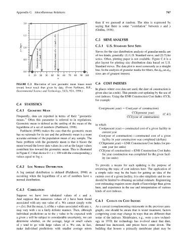
FIGURE C.3 Illustration of how geometric mean biases result C.6 COST INDEXES
toward lower result than given by data. (From Parkhurst, D.F.,
In places where cost data are used, the date of construction is
Environmental Science and Technology, 32(3), 92A, 1998.)
given also (as a rule). This permits cost updating by the use of
cost indexes. Using the ENR Construction Cost Index (CCI),
for example
C.4 STATISTICS
Cost(present year) ¼ Cost(year of construction)
C.4.1 GEOMETRIC MEAN
CCI(present year) (C:41)
Frequently, data are reported in terms of their ‘‘geometric CCI(year of construction)
means.’’ Often this parameter is referred to in regulations.
Geometric mean is defined as the antilog of the mean of the
in which
logarithms of a set of numbers (Parkhurst, 1998).
Cost(present year) ¼ constructed cost of a given facility in
Parkhurst (1998) makes the case that the geometric mean
current year
has no rationale for its use and the arithmetic mean is a more
Cost(year of construction) ¼ constructed cost of a given
accurate estimate of the population mean of any sample. The
facility in year construction was completed (dollars)
basic problem with the geometric mean is that it biases the
CCI(present year) ¼ ENR Construction Cost Index for pre-
mean toward the lower data values in a set as the larger values
sent year (no units)
contribute less toward the geometric mean. This is illustrated
CCI(year of construction) ¼ ENR Construction Cost Index
in Figure C.3 that shows 0 < x < 100 with the corresponding y
for year construction was completed for the given facil-
values equal to log x.
ity (no units)
To provide a means for such updating is the purpose of
C.4.2 LOG NORMAL DISTRIBUTION
reviewing the topic of cost indexes here. The application of
A log normal distribution is defined (Parkhurst, 1998) as a simple ratio may be the basis for getting an idea of the
occurring when the logarithms of a set of numbers have a current cost of a given facility, it is also simplistic and its use
normal distribution. should be limited to obtaining an initial estimate. Engineering
cost estimating requires more depth of knowledge than given
here, and experience in the use and interpretation of various
C.4.3 CORRELATION
kinds of cost indexes.
Suppose we have two tabulated values of x and y.
And suppose that numerous values of y have been found
C.6.1 CAVEATS ON COST INDEXES
associated with any one value of x. We cannot simply write
y ¼ f(x). But the mean, y, of the y values associated with any x, As a caveat (complementing statements in the previous para-
may vary with x in a fairly definite manner. Then, although graph), one should be aware that in water treatment, factors
individual predictions as to the y value to be expected with comprising costs may change in ways that are different than
a given x will be subject to considerable uncertainty, we can some of the indexes. Membranes, e.g., were a new technol-
determine whether, on the average, large or small values ogy in 1970; the technology has evolved since that date,
of y tend to go with large values of x. We can, in fact, demand has increased, and prices have come down. The
make individual predictions with smaller average errors building that houses a primarily membrane plant may be