Page 840 - Fundamentals of Water Treatment Unit Processes : Physical, Chemical, and Biological

Appendix D: Fluid Mechanics—Reviews of Selected Topics 795

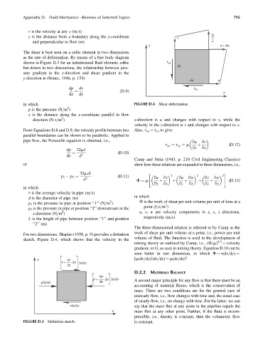
v is the velocity at any y (m=s)
y is the distance from a boundary along the y-coordinate v v +Δv
and perpendicular to flow (m)
y u +Δu
The shear is best seen on a cubic element in two dimensions
as the rate of deformation. By means of a free body diagram
shown in Figure D.3 for an infinitesimal fluid element, cubic τ yx
dy
but drawn in two dimensions, the relationship between pres-
sure gradient in the x-direction and shear gradient in the
y-direction is (Rouse, 1946, p. 154)
dx u
dp dt τ xy
(D:9) x
dx dy
¼
in which FIGURE D.4 Shear deformation.
2
p is the pressure (N=m )
x is the distance along the x-coordinate parallel to flow
2
direction (N s=m ) x-direction is u and changes with respect to y, while the
velocity in the y-direction is v and changes with respect to x.
From Equations D.8 and D.9, the velocity profile between two Also, t yx ¼ t xy to give
parallel boundaries can be shown to be parabolic. Applied to
pipe flow, the Poiseuille equation is obtained, i.e., qu qv
t yx ¼ t xy ¼ m þ (D:12)
qy qx
dp 32mv
(D:10)
dx d 2
¼
Camp and Stein (1943, p. 210 Civil Engineering Classics)
or show how these relations are expanded to three dimensions, i.e.,
32mvL " #
(D:11) 2 2 2
d F ¼ m (D:13)
p 1 p 2 ¼ 2 qu qv qu qw qv qw
qy þ qx þ qz þ qx þ qz þ qy
in which
v is the average velocity in pipe (m=s)
in which
d is the diameter of pipe (m)
2
p 1 is the pressure in pipe at position ‘‘1’’ (N=m ) F is the work of shear per unit volume per unit of time at a
3
point (J=s=m )
p 2 is the pressure in pipe at position ‘‘2’’ downstream in the
2
x-direction (N=m ) u, v, w are velocity components in x, y, z directions,
respectively (m=s)
L is the length of pipe between position ‘‘1’’ and position
‘‘2’’ (m)
The three-dimensional relation is referred to by Camp as the
work of shear per unit volume at a point, i.e., power per unit
For two dimensions, Shapiro (1958, p. 9) provides a definition
volume of fluid. The function is used in the development of
sketch, Figure D.4, which shows that the velocity in the
mixing theory as outlined by Camp, i.e., (F=m) 0.5 ¼ velocity
gradient, or G, as seen in mixing theory. Equation D.10 can be
seen better in one dimension, in which F ¼ t(dv=dy) ¼
2
y dτ [m(dv=dy)](dv=dy) ¼ m(dv=dy) .
τ + Δy ΔxΔz
dy
D.2.2 MATERIALS BALANCE
dp
p + Δx ΔyΔz A second major principle for any flow is that there must be an
pΔyΔz dx
accounting of material fluxes, which is the conservation of
mass. There are two conditions are for the general case of
unsteady flow, i.e., flow changes with time and, the usual case
of steady flow, i.e., no change with time. For the latter, we can
τΔxΔz say that the mass flux at any point in the pipeline equals the
x mass flux at any other point. Further, if the fluid is incom-
pressible, i.e., density is constant, then the volumetric flow
FIGURE D.3 Definition sketch. is constant.