Page 223 - Geochemical Anomaly and Mineral Prospectivity Mapping in GIS

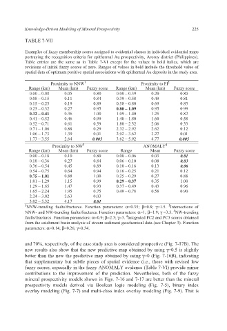
Knowledge-Driven Modeling of Mineral Prospectivity 225

TABLE 7-VII

Examples of fuzzy membership scores assigned to evidential classes in individual evidential maps
portraying the recognition criteria for epithermal Au prospectivity, Aroroy district (Philippines).
Table entries are the same as in Table 7-VI except for the values in bold italics, which are
revisions of initial fuzzy scores of zero. Ranges of values in bold include the threshold value of
spatial data of optimum positive spatial associations with epithermal Au deposits in the study area.

2
Proximity to NNW 1 Proximity to FI
Range (km) Mean (km) Fuzzy score Range (km) Mean (km) Fuzzy score
0.00 – 0.08 0.05 0.80 0.00 – 0.39 0.20 0.80
0.08 – 0.15 0.11 0.84 0.39 – 0.58 0.49 0.81
0.15 – 0.23 0.19 0.89 0.58 – 0.80 0.69 0.83
0.23 – 0.32 0.27 0.95 0.80 – 1.09 0.95 0.99
0.32 – 0.41 0.36 1.00 1.09 – 1.40 1.25 0.82
0.41 – 0.52 0.46 0.99 1.40 – 1.80 1.60 0.58
0.52 – 0.71 0.61 0.59 1.80 – 2.32 2.06 0.33
0.71 – 1.06 0.88 0.29 2.32 – 2.92 2.62 0.12
1.06 – 1.73 1.39 0.01 2.92 – 3.62 3.27 0.01
1.73 – 3.55 2.64 0.005 3.62 – 5.92 4.77 0.005
4
Proximity to NW 3 ANOMALY
Range (km) Mean (km) Fuzzy score Range Mean Fuzzy score
0.00 – 0.18 0.10 0.80 0.00 – 0.06 0.03 0.01
0.18 – 0.36 0.27 0.84 0.06 – 0.10 0.08 0.03
0.36 – 0.54 0.45 0.89 0.10 – 0.16 0.13 0.06
0.54 – 0.75 0.64 0.94 0.16 – 0.25 0.21 0.12
0.75 – 1.01 0.88 1.00 0.25 – 0.29 0.27 0.88
1.01 – 1.29 1.15 0.99 0.29 – 0.37 0.35 1.00
1.29 – 1.65 1.47 0.93 0.37 – 0.49 0.43 0.96
1.65 – 2.24 1.95 0.75 0.49 – 0.78 0.58 0.90
2.24 – 3.02 2.63 0.03
3.02 – 5.32 4.17 0.01
1 NNW-trending faults/fractures. Function parameters: α=0.35; β=0.8; γ=1.5. Intersections of
2
3
NNW- and NW-trending faults/fractures. Function parameters: α=1; β=1.9; γ =3.5. NW-trending
4
faults/fractures. Function parameters: α=0.9; β=2.3; γ=3. Integrated PC2 and PC3 scores obtained
from the catchment basin analysis of stream sediment geochemical data (see Chapter 3). Function
parameters: α=0.14; β=0.26; γ=0.34.

and 70%, respectively, of the case study area is considered prospective (Fig. 7-17B). The
new results also show that the new predictive map obtained by using γ=0.5 is slightly
better than the new the predictive map obtained by using γ=0 (Fig. 7-16B), indicating
that supplementary but subtle pieces of spatial evidence (i.e., those with revised low
fuzzy scores, especially in the fuzzy ANOMALY evidence (Table 7-VI) provide minor
contributions to the improvement of the prediction. Nevertheless, both of the fuzzy
mineral prospectivity models shown in Figs. 7-16 and 7-17 are better than the mineral
prospectivity models derived via Boolean logic modeling (Fig. 7-5), binary index
overlay modeling (Fig. 7-7) and multi-class index overlay modeling (Fig. 7-9). That is