Page 133 - Geometric Modeling and Algebraic Geometry

134 T. Beck and J. Schicho
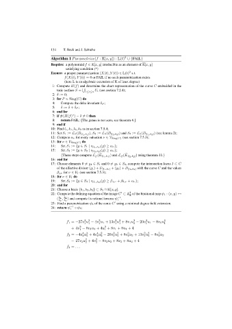
Algorithm 1 Parametrize(f : K[x, y]) : L(t) ∪{FAIL}
2
Require: a polynomial f ∈ K[x, y] irreducible as an element of K[x, y]
satisfying condition (*)
Ensure: a proper parametrization (X(t),Y (t)) ∈ L(t) s.t.
2
f(X(t),Y (t)) = 0 or FAIL if no such parametrization exists
(here L is an algebraic extension of K of least degree)
1: Compute Π(f) and determine the chart representation of the curve C embedded in the

toric surface S = 1≤i≤n U i (see section 7.2.4);
2: δ := 0;
3: for P ∈ Sing(C) do
4: Compute the delta invariant δ P ;
5: δ := δ + δ P ;
6: end for
7: if #(Π(f) ) − δ =0 then
◦
8: return FAIL; {The genus is not zero, see theorem 4.}
9: end if
10: Find l 1,k 1,l 2,k 2 as in section 7.5.4;
11: Set S 1 := L S(D [l 1 ,k 1 ] ), S 2 := L S(D [l 2 ,k 2 ] ) and S 3 := L S(D [l 1 ,k 2 ] ) (see lemma 2);
12: Compute α ν for every valuation ν ∈V Sing(C) (see section 7.5.3);
13: for ν ∈V Sing(C) do
14: Set S 1 := {g ∈ S 1 | ν [l 1 ,k 1 ] (g) ≥ α ν };
15: Set S 2 := {g ∈ S 2 | ν [l 2 ,k 2 ] (g) ≥ α ν };

{These steps compute L C (K [l 1 ,k 1 ] ) and L C (K [l 2 ,k 2 ] ) using theorem 11.}
16: end for
17: Choose elements 0 = g 1 ∈ S 1 and 0 = g 2 ∈ S 2, compute the intersection locus I ⊂ C
of the effective divisor (g 1)+ D [l 1 ,k 1 ] +(g 2)+ D [l 2 ,k 2 ] with the curve C and the values
β j,ν for ν ∈V I (see section 7.5.3);
18: for ν ∈V I do
19: Set S 3 := {g ∈ S 3 | ν [l 1 ,k 2 ] (g) ≥ β 1,ν + β 2,ν + α ν };
20: end for
21: Choose a basis {b 1,b 2,b 3}⊂ S 3 ∩ K[x, y].
2
22: Compute the defining equation of the image C ⊂ A of the birational map ψ 1 :(x, y) →
K
( b 1 , b 2 ) and compute its rational inverse ψ −1 .
1
b 3
b 3

23: Find a parametrization ψ 2 of the conic C using a minimal degree field extension.
24: return ψ −1 ◦ ψ 2;
1
f 1 = −27v u − 4v u 1 +13v u +8v 1 u − 20v u 1 − 8v 1 u 2
2 3
3
3
2
2 2
1 1 1 1 1 1 1 1
+4v − 8v 1 u 1 +4u +8v 1 +8u 1 +4
2
2
1 1
4 3 4 2 3 2 3 2 2 2
f 2 = −4v u +4v u − 20v u +8v u 2 +13v u − 8v u 2
2 2 2 2 2 2 2 2 2 2
− 27v 2 u +4v − 8v 2 u 2 +8v 2 +8u 2 +4
2
2
2 2
f 3 = ...