Page 162 - Geometric Modeling and Algebraic Geometry

164 S. Chau et al.
In our application to surface–surface–intersections, the resultant can be used as
a projection operator. Indeed, if f 1 ,f 2 and f 3 are the three components of x(u, v) −
y(r, s) which are considered as polynomials in the two variables r and s, then the
resultant of f 1 ,f 2 and f 3 is a polynomial R(u, v) and it gives an implicit plane curve
which corresponds to the projection of C in the (u, v) parameters. More precisely, if
f 1 ,f 2 and f 3 are generic, then the two sets
$ %
(u, v) ∈ [0, 1] | R(u, v)=0 (9.6)
2
and
$ %
(u, v) ∈ [0, 1] |∃(r, s) ∈D : x(u, v)= y(r, s) (9.7)
2
are identical. Several families of multivariate resultants have been studied and some
implementations are available, see [5, 22].

9.3.2 Application to the intersection problem

A strategy to describe the intersection between x(u, v) and y(r, s) consists in pro-
jecting C on a plane (by using the resultant). Many authors propose to project C on the
(u, v) (or (r, s)) plane and then the resulted plane curve is traced (see [16] and [20]
for the tracing method) and is lifted to the 3D space by the corresponding parame-
terization. Note that this method can give some unwanted components (the so called
“phantom components”) which are not in x([0, 1] ) ∩ y([0, 1] ). So, another step is
2
2
needed to cut off the extraneous branches. This last part can be done with a solver for
multivariate polynomial systems (see [25]) or an inversion of parameterization (see
[3]).
As an alternative to these existing approaches, we propose to project the set C
onto the (u, r) space. Note that, in the equations x(u, v)= y(r, s), the two variables
v and s are separated, so they can be eliminated via a simple resultant computation.
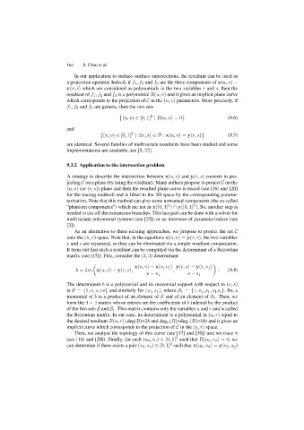
It turns out that such a resultant can be computed via the determinant of a Bezoutian
matrix (see [15]). First, consider the (3, 3) determinant:

x(u, v) − x(u, v 1 ) y(r, s) − y(r, s 1 )
b =det x(u, v) − y(r, s), v − v 1 , s − s 1 . (9.8)

The determinant b is a polynomial and its monomial support with respect to (v, s)
is S = {1,v,s,vs} and similarly for (v 1 ,s 1 ), where S 1 = {1,v 1 ,s 1 ,v 1 s 1 }. So, a
monomial of b is a product of an element of S and of an element of S 1 . Then, we
form the 4 × 4 matrix whose entries are the coefficients of b indexed by the product
of the two sets S and S 1 . This matrix contains only the variables u and r and is called
the Bezoutian matrix. In our case, its determinant is a polynomial in (u, r) equal to
the desired resultant R(u, r) (deg(R)=24 and deg u (R)=deg r (R)=16) and it gives an
implicit curve which corresponds to the projection of C in the (u, r) space.
Then, we analyse the topology of this curve (see [17] and [30]) and we trace it
(see [16] and [20]). Finally, for each (u 0 ,r 0 ) ∈ [0, 1] such that R(u 0 ,r 0 )=0,we
2
can determine if there exists a pair (v 0 ,s 0 ) ∈ [0, 1] such that x(u 0 ,v 0 )= y(r 0 ,s 0 )
2