Page 161 - Geometric Modeling and Algebraic Geometry

9 Intersecting Biquadratic Patches 163
v

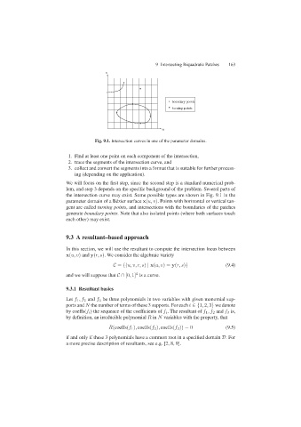
boundary points
turning points

u
Fig. 9.1. Intersection curves in one of the parameter domains.

1. Find at least one point on each component of the intersection,
2. trace the segments of the intersection curve, and
3. collect and convert the segments into a format that is suitable for further process-
ing (depending on the application).

We will focus on the first step, since the second step is a standard numerical prob-
lem, and step 3 depends on the specific background of the problem. Several parts of
the intersection curve may exist. Some possible types are shown in Fig. 9.1 in the
parameter domain of a B´ ezier surface x(u, v). Points with horizontal or vertical tan-
gent are called turning points, and intersections with the boundaries of the patches
generate boundary points. Note that also isolated points (where both surfaces touch
each other) may exist.

9.3 A resultant–based approach

In this section, we will use the resultant to compute the intersection locus between
x(u, v) and y(r, s). We consider the algebraic variety

C = {(u, v, r, s) | x(u, v)= y(r, s)} (9.4)
and we will suppose that C∩ [0, 1] is a curve.
4

9.3.1 Resultant basics
Let f 1 ,f 2 and f 3 be three polynomials in two variables with given monomial sup-
ports and N the number of terms of these 3 supports. For each i ∈{1, 2, 3} we denote
by coeffs(f i ) the sequence of the coefficients of f i . The resultant of f 1 ,f 2 and f 3 is,
by definition, an irreducible polynomial R in N variables with the property, that
R(coeffs(f 1 ), coeffs(f 2 ), coeffs(f 3 )) = 0 (9.5)

if and only if these 3 polynomials have a common root in a specified domain D.For
a more precise description of resultants, see e.g. [2, 8, 9].