Page 165 - Geometric Modeling and Algebraic Geometry

9 Intersecting Biquadratic Patches 167

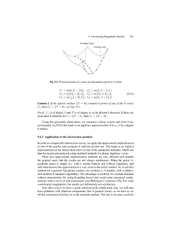
Fig. 9.3. Characterization of a conic in a biquadratic patch by 9 points

C 1 = x([0, 1] ×{0}),C 2 = x([0, 1] ×{1})
C 3 = x({0}× [0, 1]),C 4 = x({1}× [0, 1]) (9.11)
C 5 = x({ }× [0, 1]),C 6 = x([0, 1] ×{ })
1
1
2 2
Lemma 1. If the quartic surface {P =0} contains 9 points of any of the 6 conics
C i , then C i ⊂{P =0}, see Fig. 9.3.
Proof. C i is of degree 2 and P is of degree 4, so by B´ ezout’s theorem, if there are
more than 8 elements in C i ∩{P =0}, then C i ⊂{P =0}.
Using this geometric observation, we construct a linear system and solve it ap-
proximately via SVD; this leads to an algebraic approximation of x(u, v) by a degree
4 surface.

9.4.3 Application to the intersection problem

In order to compute the intersection curves, we apply the approximate implicitization
to one of the patches and compose it with the second one. This leads to an implicit
representation of the intersection curve in one of the parameter domains, which can
then be traced and analyzed using standard methods for planar algebraic curves.
These two approximate implicitization methods are very efficient and suitable
for general cases, but the results are not always satisfactory. When the given bi-
quadratic patch is simple (i.e. with a certain flatness and without singularity and
self–intersection) the approximation is very close to the initial surface. So, to use this
method for a general biquadratic surface, we combine it, if needed, with a subdivi-
sion method (Casteljau’s algorithm). The advantage is twofold, we exclude domains
without intersections (by using bounding boxes) and avoid some unwanted config-
urations with a curve of self-intersection (use Hohmeyer’s criterion [19]). For more
complicated singularities, the results are definitively not satisfactory.
Note that even if we have a good criterion in the subdivision step, we still may
have problems with phantom components (but in general fewer), so we have to cut
off the extraneous branches as in the resultant method. This has to be done carefully