Page 169 - Geometric Modeling and Algebraic Geometry

9 Intersecting Biquadratic Patches 171
Intersection of the cylinder and the intersection curves.

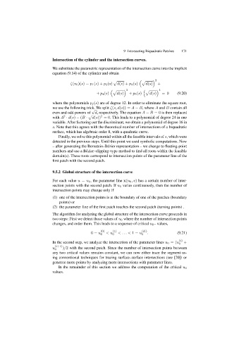
We substitute the parametric representation of the intersection curve into the implicit
equation (9.14) of the cylinder and obtain

& & 2
ζ(u 0 )(s)= p 1 (s)+ p 2 (s) d(s)+ p 3 (s) d(s) +

& 3 & 4
+ p 4 (s) d(s) + p 5 (s) d(s) =0 (9.20)
where the polynomials p j (s) are of degree 12. In order to eliminate the square root,
we use the following trick. We split ζ(s, d(s)) = A − B, where A and B contain all
√
even and odd powers of d, respectively. The equation A − B =0 is then replaced
&
with A · d(s) − (B · d(s)) =0. This leads to a polynomial of degree 24 in one
2
2
variable. After factoring out the discriminant, we obtain a polynomial of degree 16 in
s. Note that this agrees with the theoretical number of intersections of a biquadratic
surface, which has algebraic order 8, with a quadratic curve.
Finally, we solve this polynomial within all the feasible intervals of s, which were
detected in the previous steps. Until this point we used symbolic computations. Now
– after generating the Bernstein–B´ ezier representation – we change to floating-point
numbers and use a B´ ezier–clipping–type method to find all roots within the feasible
domain(s). These roots correspond to intersection points of the parameter line of the
first patch with the second patch.

9.5.2 Global structure of the intersection curve

For each value u = u 0 , the parameter line x(u 0 ,v) has a certain number of inter-
section points with the second patch. If u 0 varies continuously, then the number of
intersection points may change only if
(1) one of the intersection points is at the boundary of one of the patches (boundary
points) or
(2) the parameter line of the first patch touches the second patch (turning points) .
The algorithm for analyzing the global structure of the intersection curve proceeds in
two steps: First we detect those values of u 0 where the number of intersection points
changes, and order them. This leads to a sequence of critical u 0 – values,

0= u (0) <u (1) < ... < 1= u (K) . (9.21)
0 0 0
In the second step, we analyze the intersection of the parameter lines u 0 =(u (i) +
0
u (i+1) )/2 with the second patch. Since the number of intersection points between
0
any two critical values remains constant, we can now either trace the segment us-
ing conventional techniques for tracing surface–surface intersections (see [20]) or
generate more points by analyzing more intersections with parameter lines.

In the remainder of this section we address the computation of the critical u 0
values.