Page 173 - Geometric Modeling and Algebraic Geometry

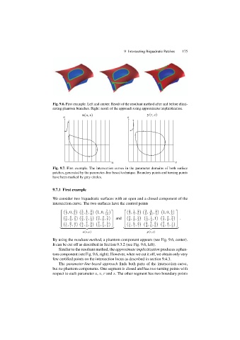
9 Intersecting Biquadratic Patches 175

Fig. 9.6. First example. Left and center: Result of the resultant method after and before elimi-
nating phantom branches. Right: result of the approach using approximate implicitization.
x(u, v) y(r, s)
v s

u r
Fig. 9.7. First example. The intersection curves in the parameter domains of both surface
patches, generated by the parameter–line based technique. Boundary points and turning points
have been marked by grey circles.

9.7.1 First example

We consider two biquadratic surfaces with an open and a closed component of the
intersection curve. The two surfaces have the control points

⎡ ⎤ ⎡ ⎤
, 0, , , 1, 0, , , , , 1, 0,
1 3 3 1 3 7 2 1 2 3 1 2 4
7 5 5 5 4 10 7 7 5 5 10 3 5

⎢ 6 3 5 ⎥ ⎢ 5 3 2 ⎥
, ,
, , 1
, ,
, ,
3 4 2 2 3 1 , , 3 4 2 1 1 , , ⎦ .
⎣ ⎦ and ⎣
8 9 3 3 4 3 7 8 7 8 9 3 3 2 7 8 7

, , , , , , , , , , , ,
1 6 4 3 7 3 7 7 5 1 6 3 3 7 5 7 4 1
5 7 7 4 8 4 8 9 8 5 7 7 4 8 8 8 7 2

x(u,v) y(r,s)
By using the resultant method, a phantom component appears (see Fig. 9.6, center).
It can be cut off as described in Section 9.3.2 (see Fig. 9.6, left).
Similar to the resultant method, the approximate implicitization produces a phan-
tom component (see Fig. 9.6, right). However, when we cut it off, we obtain only very
few certified points on the intersection locus as described in section 9.4.3.
The parameter-line-based approach finds both parts of the intersection curve,
but no phantom components. One segment is closed and has two turning points with
respect to each parameter u, v, r and s. The other segment has two boundary points