Page 172 - Geometric Modeling and Algebraic Geometry

174 S. Chau et al.

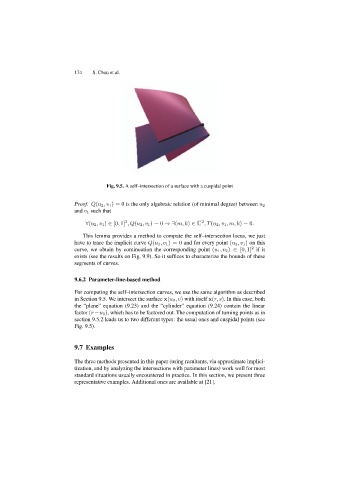
Fig. 9.5. A self–intersection of a surface with a cuspidal point

Proof. Q(u 2 ,v 1 )=0 is the only algebraic relation (of minimal degree) between u 2
and v 1 such that

∀(u 2 ,v 1 ) ∈ [0, 1] ,Q(u 2 ,v 1 )=0 ⇒∃(m, k) ∈ 2 ,T(u 2 ,v 1 ,m,k)=0.
2
This lemma provides a method to compute the self–intersection locus, we just
have to trace the implicit curve Q(u 2 ,v 1 )=0 and for every point (u 2 ,v 1 ) on this
curve, we obtain by continuation the corresponding point (u 1 ,v 2 ) ∈ [0, 1] if it
2
exists (see the results on Fig. 9.9). So it suffices to characterize the bounds of these
segments of curves.

9.6.2 Parameter-line-based method

For computing the self–intersection curves, we use the same algorithm as described
in Section 9.5. We intersect the surface x(u 0 ,v) with itself x(r, s). In this case, both
the “plane” equation (9.23) and the “cylinder” equation (9.24) contain the linear
factor (r−u 0 ), which has to be factored out. The computation of turning points as in
section 9.5.2 leads us to two different types: the usual ones and cuspidal points (see
Fig. 9.5).

9.7 Examples

The three methods presented in this paper (using resultants, via approximate implici-
tization, and by analyzing the intersections with parameter lines) work well for most
standard situations usually encountered in practice. In this section, we present three
representative examples. Additional ones are available at [21].