Page 174 - Geometric Modeling and Algebraic Geometry

176 S. Chau et al.
u =0 and s =1 and also possesses a turning point with respect to v and another one
with respect to r (see Fig. 9.7).

9.7.2 Second example

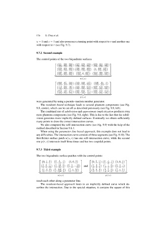
The control points of the two biquadratic surfaces
⎡ ⎤
, , , , , ,
501 388 588 347 276 479 309 604 498
775 775 775 775 775 775 775 775 775

⎢ ⎥
,
,
,
,
,
553 454 293 336 382 469 1, 426 137
⎣ ⎦
775 775 775 775 775 775 775 775

, , , 0, , ,
337 308 258 517 367 533 492 564
775 775 775 775 775 775 775 775

x(u,v)
⎡ ⎤
, , , , , ,
492 67 522 543 322 117 346 13 4
775 155 775 775 775 775 775 155 5

⎢ 307 514 564 ⎥
,
,
,
113 392 , 58 632 469 413 , ,
⎣ ⎦
155 775 155 775 775 775 775 775 775

, , , , , ,
602 129 274 669 692 53 488 219 412
775 775 775 775 775 155 775 775 775

y(r,s)
were generated by using a pseudo–random number generator.
The resultant–based technique leads to several phantom components (see Fig.
9.8, center), which can be cut off as described previously (see Fig. 9.8, left).
The combined use of subdivision and approximate implicitization produces even
more phantom components (see Fig. 9.8, right). This is due to the fact that the subdi-
vision generates more implicitly defined surfaces. Eventually we obtain sufficiently
many points to draw the correct intersection curves.
We also computed the self–intersection curve (see Fig. 9.9) with the help of the
method described in Section 9.6.1.
When using the parameter–line based approach, this example does not lead to
any difficulties. The intersection curve consists of three segments (see Fig. 9.10). The
first B´ ezier surface patch x(u, v) has one self–intersection curve, while the second
one y(r, s) intersects itself three times and has two cuspidal points.
9.7.3 Third example
The two biquadratic surface patches with the control points
⎡ ⎤ ⎡ ⎤
0, , 3 , 1 , 1 1, 0, 4 0, , 3 , 1 , 1 1, 0, 1
1 4
1 1
7 5 5 13 3 5 7 5 5 10 3 5

,
, ,
⎢ 16 ⎥ ⎢ 6 3 1 ⎥
, ,
, ,
,
1 4 11 1 34 3 6 3 1 4 7 1 1 3 , ,
⎣ , , − ⎦ and ⎣ ⎦
8 9 40 3 65 4 7 8 35 8 9 8 3 2 4 7 8 7

, , , , , 1, , , , , , 1,
1 6 4 3 443 3 7 14 1 6 1 3 7 3 7 1
5 7 5 4 520 8 8 15 5 7 5 4 8 8 8 3

x(u,v) y(r,s)
touch each other along a parameter line.
The resultant-based approach leads to an implicitly defined curve which de-
scribes the intersection. Due to the special situation, it contains the square of this