Page 166 - Geometric Modeling and Algebraic Geometry

168 S. Chau et al.
π 1
r

x(u, v)
π r 1 k π 2

ζ

k π 2
k π 1
s
s 0
s 1
π 2
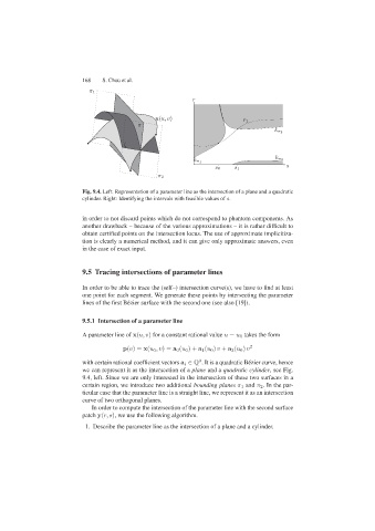
Fig. 9.4. Left: Representation of a parameter line as the intersection of a plane and a quadratic
cylinder. Right: Identifying the intervals with feasible values of s.

in order to not discard points which do not correspond to phantom components. As
another drawback – because of the various approximations – it is rather difficult to
obtain certified points on the intersection locus. The use of approximate implicitiza-
tion is clearly a numerical method, and it can give only approximate answers, even
in the case of exact input.

9.5 Tracing intersections of parameter lines

In order to be able to trace the (self–) intersection curve(s), we have to find at least
one point for each segment. We generate these points by intersecting the parameter
lines of the first B´ ezier surface with the second one (see also [19]).

9.5.1 Intersection of a parameter line

A parameter line of x(u, v) for a constant rational value u = u 0 takes the form
p(v)= x(u 0 ,v)= a 0 (u 0 )+ a 1 (u 0 ) v + a 2 (u 0 ) v 2

with certain rational coefficient vectors a i ∈ Q . It is a quadratic B´ ezier curve, hence
3
we can represent it as the intersection of a plane and a quadratic cylinder, see Fig.
9.4, left. Since we are only interested in the intersection of these two surfaces in a
certain region, we introduce two additional bounding planes π 1 and π 2 . In the par-
ticular case that the parameter line is a straight line, we represent it as an intersection
curve of two orthogonal planes.
In order to compute the intersection of the parameter line with the second surface
patch y(r, s), we use the following algorithm.
1. Describe the parameter line as the intersection of a plane and a cylinder.