Page 250 - Global Tectonics

236 CHAPTER 8

38 N 36 N
(a) 244 246 34 (b)
242
40 SAF ECSZ
North America Plate 32 30
Velocity (mm a -1 ) 20
38 246 10
240
0 North profile SAF
40
Velocity (mm a -1 ) 30

20
30 244 10
238
Pacific Plate 25 mm a -1 South profile SJF
0 0 100 200 300 400 500
36 238 34 240 32 242 30 Distance (km)
(c) (d)
38 244 36 246 34 242 38 244 36 246 34
242
North America Plate
Furnace Creek
Furnace Creek Valley North America Plate 32 32
Death
Death
Valley
Panamint Valley
Panamint Valley
38 Owens Valley Imperial 246 38 246
Owens Valley
Imperial
San Jacinto 240
San Jacinto
240
Mojave SAF
Garlock Garlock Mojave SAF
Elsinore
Elsinore
Newport-Inglewood-Rose Canyon
Newport-Inglewood-Rose Canyon
Agua Blanca
Agua Blanca
San Andreas
San Andreas
Palos Verdes
Palos Verdes 244 244
238
Pacific Plate 30 238 5 mm a -1 30

36 238 34 240 32 242 30 36 238 34 240 32 242 30
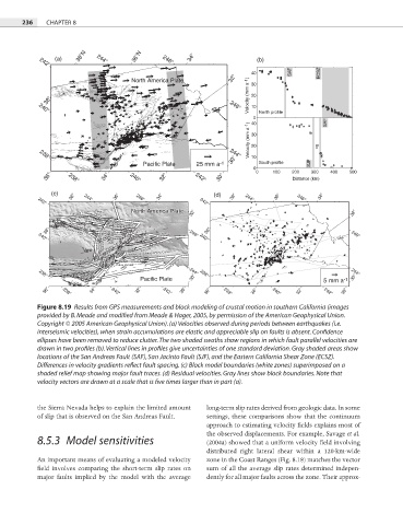
Figure 8.19 Results from GPS measurements and block modeling of crustal motion in southern California (images

provided by B. Meade and modified from Meade & Hager, 2005, by permission of the American Geophysical Union.
Copyright © 2005 American Geophysical Union). (a) Velocities observed during periods between earthquakes (i.e.

interseismic velocities), when strain accumulations are elastic and appreciable slip on faults is absent. Confidence
ellipses have been removed to reduce clutter. The two shaded swaths show regions in which fault parallel velocities are

drawn in two profiles (b). Vertical lines in profiles give uncertainties of one standard deviation. Gray shaded areas show

locations of the San Andreas Fault (SAF), San Jacinto Fault (SJF), and the Eastern California Shear Zone (ECSZ).

Differences in velocity gradients reflect fault spacing. (c) Block model boundaries (white zones) superimposed on a
shaded relief map showing major fault traces. (d) Residual velocities. Gray lines show block boundaries. Note that
velocity vectors are drawn at a scale that is five times larger than in part (a).

the Sierra Nevada helps to explain the limited amount long-term slip rates derived from geologic data. In some
of slip that is observed on the San Andreas Fault. settings, these comparisons show that the continuum
approach to estimating velocity fields explains most of

the observed displacements. For example, Savage et al.
8.5.3 Model sensitivities (2004a) showed that a uniform velocity fi eld involving
distributed right lateral shear within a 120-km-wide
An important means of evaluating a modeled velocity zone in the Coast Ranges (Fig. 8.18) matches the vector
field involves comparing the short-term slip rates on sum of all the average slip rates determined indepen-

major faults implied by the model with the average dently for all major faults across the zone. Their approx-