Page 59 - Global Tectonics

46 CHAPTER 2

of such a feature is small in the central part of the
plateau so that here the Bouguer anomaly, BA, is related
to the free-air anomaly, FAA by the relationship:

BA = FAA − BC

where BC is the Bouguer correction, equal to 2πGρ c h,
where ρ c is the density of the compensated layer. For
such an Airy compensation:

IA = BA − A root
where A root is the gravity anomaly of the compensating
root. Since the root is broad compared to its thickness,
its anomaly may be approximated by that of an infi nite
slab, that is 2πG(ρ c − ρ m )r, where ρ m is the density of
the substrate. Combining the above two equations:

IA = FAA − 2πGρ c h − 2πG(ρ c − ρ m )r

From the Airy criterion for isostatic equilibrium:

r = hρ c /(ρ m − ρ c )

Substitution of this condition into the equation reveals
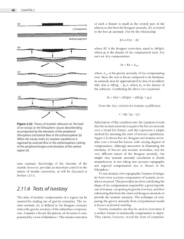
Figure 2.32 Theory of isostatic rebound. (a) The load
that the isostatic anomaly is equal to the free-air anomaly
of an icecap on the lithosphere causes downbending

over a broad flat feature, and this represents a simple
accompanied by the elevation of the peripheral
method for assessing the state of isostatic equilibrium.
lithosphere and lateral flow in the asthenosphere (b).

Figure 2.33 shows free-air, Bouguer and isostatic anom-
When the icecap melts (c), isostatic equilibrium is

regained by reversed flow in the asthenosphere, sinking alies over a broad flat feature with varying degrees of
of the peripheral bulges and elevation of the central compensation. Although instructive in illustrating the
region (d). similarity of free-air and isostatic anomalies, and the
very different nature of the Bouguer anomaly, this
simple Airy isostatic anomaly calculation is clearly
unsatisfactory in not taking into account topography
time constant. Knowledge of the viscosity of the

and regional compensation due to flexure of the
mantle, however, provides an important control on the
lithosphere.
nature of mantle convection, as will be discussed in
To test isostasy over topographic features of irregu-
Section 12.5.2.
lar form more accurate computation of isostatic anom-
alies is required. This procedure involves calculating the
shape of the compensation required by a given hypoth-
2.11.6 Tests of isostasy esis of isostasy, computing its gravity anomaly, and then
subtracting this from the observed Bouguer anomaly to
The state of isostatic compensation of a region can be provide the isostatic anomaly. The technique of com-
assessed by making use of gravity anomalies. The iso- puting the gravity anomaly from a hypothetical model

static anomaly, IA, is defined as the Bouguer anomaly is known as forward modeling.
minus the gravity anomaly of the subsurface compensa- Gravity anomalies can thus be used to determine if
tion. Consider a broad, flat plateau of elevation h com- a surface feature is isostatically compensated at depth.

pensated by a root of thickness r. The terrain correction They cannot, however, reveal the form of compensa-