Page 63 - Global Tectonics

50 CHAPTER 2

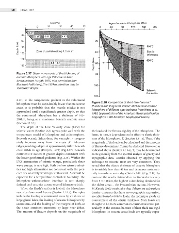
Figure 2.37 Shear wave model of the thickening of
−1
oceanic lithosphere with age. Velocities in km s
(redrawn from Forsyth, 1975, with permission from
Blackwell Publishing). The 150 km transition may be
somewhat deeper.

2.13), so the temperature gradient in the sub-crustal
lithosphere must be considerably lower than in oceanic Figure 2.38 Comparison of short-term “seismic”
thickness and long-term “elastic” thickness for oceanic
areas. It is probable that the mantle solidus is not

approached until a significantly greater depth, so that lithosphere of different ages (redrawn from Watts et al.,
1980, by permission of the American Geophysical Union.
the continental lithosphere has a thickness of 100– Copyright © 1980 American Geophysical Union).
250 km, being at a maximum beneath cratonic areas
(Section 11.3.1).
The depth of the Low Velocity Zone (LVZ) for

seismic waves (Section 2.2) agrees quite well with the the load and the flexural rigidity of the lithosphere. The
temperature model of lithosphere and asthenosphere. latter, in turn, is dependent on the effective elastic thick-
Beneath oceanic lithosphere, for example, it progres- ness of the lithosphere, T e (Section 2.11.4). Thus, if the
sively increases away from the crests of mid-ocean magnitude of the load can be calculated and the amount
ridges, reaching a depth of approximately 80 km beneath of fl exure determined, T e may be deduced. However as
crust 80 Ma in age (Forsyth, 1975) (Fig.2.37). Beneath indicated above (Section 2.11.6), T e may be determined
continents it occurs at greater depths consistent with more generally from the spectral analysis of gravity and
the lower geothermal gradients (Fig. 2.36). Within the topographic data. Results obtained by applying this
LVZ attenuation of seismic energy, particularly shear technique to oceanic areas are very consistent. They
wave energy, is very high. Both the low seismic veloci- reveal that the elastic thickness of oceanic lithosphere
ties and high attenuation are consistent with the pres- is invariably less than 40 km and decreases systemati-
ence of a relatively weak layer at this level. As would be cally towards oceanic ridges (Watts, 2001) (Fig. 2.38). By
expected for a temperature-controlled boundary, the contrast, the results obtained for continental areas vary
lithosphere–asthenosphere interface is not sharply from 5 to 110 km, the highest values being obtained for

defined, and occupies a zone several kilometers thick. the oldest areas – the Precambrian cratons. However,
When the Earth’s surface is loaded, the lithosphere McKenzie (2003) maintains that if there are sub-surface
reacts by downward fl exure (Section 2.11.4). Examples density contrasts that have no topographic expression,
include the loading of continental areas by ice sheets or so-called buried or hidden loads, the technique yields an
large glacial lakes, the loading of oceanic lithosphere by overestimate of the elastic thickness. Such loads are
seamounts, and the loading of the margins of both, at thought to be more common in continental areas, par-
the ocean–continent transition, by large river deltas. ticularly in the cratons, because of their thick and rigid
The amount of flexure depends on the magnitude of lithosphere. In oceanic areas loads are typically super-