Page 611 - Handbook of Battery Materials

17.4 Bulk Properties 585

association constants and related quantities and in general as a suitable source of
information on the usability of an electrolyte solution for technical application [183].
MSA is the extension of Debye-H¨ uckel theory to high electrolyte concentrations
using the same continuum model [397, 398]. Combined with the law of mass
action for ion- pair formation, MSA-MAL (mass action law approach), and finally
as associative mean spherical approximation (AMSA) [399–401], it permits us to
take into account any ion-complex formation. Equations for electrolyte conductivity
are given by Blum et al. [402, 403]. However, the complexity of battery electrolytes
hinders the application of a high concentration continuum approach.
For attempts in the literature to rationalize the maximum, with reference to
solvation, ion-association, or viscosity of the electrolyte, see Ref. [15].
The search for a suitable electrolyte requires encompassing studies. It is necessary
to measure the conductivities of electrolytes with various solvents, solvent mixtures,
and anions over accessible concentration ranges of the salts, and to cover a
sufficiently large temperature range and the whole composition range of the binary
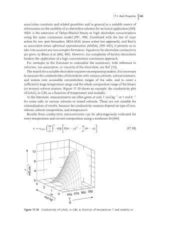
(or ternary) solvent mixture. Figure 17.10 shows an example: the conductivity plot
of LiAsF 6 in GBL as a function of temperature and molality.
In the literature, measurements are often given at only 1 mol·kg −1 or 1 mol·L −1
for some salts in various solvents or mixed solvents. These are not suitable for
rationalization of results, because the conductivity maxima depend on type of ions,
solvent, solvent composition, and temperature.
Results from conductivity measurements can be advantageously evaluated for
every temperature and solvent composition using a nonlinear fit [404]
m 2 a

a
κ = κ max · exp b(m − µ) − (m − µ) (17.48)
µ µ

12

8

k mS cm −1 4

0
3
2
1 330
m 0 240 270 300
T
mol kg
−1
K
Figure 17.10 Conductivity of LiAsF 6 in GBL as function of temperature T and molality m.