Page 302 - Handbook of Civil Engineering Calculations, Second Edition

PRESTRESSED CONCRETE 2.87

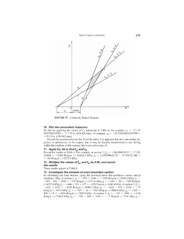
FIGURE 57. Composite Magnel diagram.

10. Plot the concordant trajectory
Do this by applying the values of C 3 appearing in Table 4; for example, e 1 21.87
(0.0550)/0.0700 17.19 in. (436.626 mm). At midspan, e m 21.87(0.0625)/0.0700
19.53 in. (496.062 mm).
Record the eccentricities on line 10 of the table. It is apparent that this concordant tra-
jectory is satisfactory in the respect that it may be linearly transformed to one falling
within the confines of the section; this is proved in step 14.
11. Apply Eq. 56 to find f bp and f tp
Record the results in Table 4. For example, at section 1, f bp 1,160,000(10.32 17.19)/
14,860 2148 lb/sq.in. ( 14,810.5 kPa); f tp 1,160,000(22.32 17.19)/32,140
185 lb/sq.in. ( 1275.6 kPa).
12. Multiply the values of f bp and f tp by 0.85, and record
the results
These results appear in Table 4.
13. Investigate the stresses at every boundary section
In calculating the final stresses, apply the live-load stress that produces a more critical
condition. Thus, at section 1, f bi 959 2148 1189 lb/sq.in. ( 8198.2 kPa); f bf
959 691 1826 176 lb/sq.in. ( 1213.6 kPa); f ti 444 185 629 lb/sq.in.
( 4337.0 kPa); f tf 444 319 157 920 lb/sq.in. ( 6343.4 kPa). At section 2: f bi
1221 2513 1292 lb/sq.in. ( 8908.3 kPa); f bf 1221 972 2136 57
lb/sq.in. ( 393.0 kPa); f ti 565 16 581 lb/sq.in. ( 4006.0 kPa); f tf 565
450 14 1029 lb/sq.in. ( 7095.0 kPa). At section 3: f bi 785 1903 1118
lb/sq.in. ( 7706.8 kPa); f bf 785 844 1618 11 lb/sq.in. ( 75.8 kPa); f ti