Page 129 - Hardware Implementation of Finite-Field Arithmetic

112 Cha pte r F o u r

elsif ce_e = ‘1’ then e <= result;
end if;
end if;
end process register_e;
register_txy: process(clk)
begin
if clk’event and clk = ‘1’ then
if ce_txy = ‘1’ then txy <= result; end if;
end if;
end process register_txy;
shift_register: process(clk)
begin
if clk’event and clk = ‘1’ then
if load = ‘1’ then int_P_MINUS_2 <= P_MINUS_2;
elsif update = ‘1’ then
for i in 1 to k-1 loop
int_P_MINUS_2(K-i) <= int_P_MINUS_2(K-i-1);
end loop;
int_P_MINUS_2(0) <= ‘0’;
end if;
end if;
end process shift_register;
ser_out <= int_P_MINUS_2(K-1);

The complete model additionally includes a (k + 1)-state counter
and a control unit.

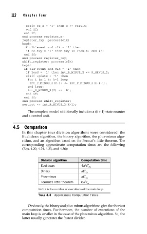
4.5 Comparison
In this chapter four division algorithms were considered: the
Euclidean algorithm, the binary algorithm, the plus-minus algo-
rithm, and an algorithm based on the Fermat’s little theorem. The
corresponding approximate computation times are the following
(Eqs. 4.20, 4.24, 4.33, and 4.36):

Division algorithm Computation time
Euclidean 4k tT
2
FA
Binary ktT
FA
Plus-minus ktT
FA
Fermat’s little theorem 6k T
2
FA
Note: t is the number of executions of the main loop.
TABLE 4.4 Approximate Computation Times

Obviously, the binary and plus-minus algorithms give the shortest
computation times. Furthermore, the number of executions of the
main loop is smaller in the case of the plus-minus algorithm. So, the
latter usually generates the fastest divider.