Page 138 - Hardware Implementation of Finite-Field Arithmetic

Operations over Z [ x ]/ f ( x ) 121
p

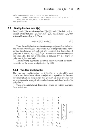
main_component: for i in 0 to M-1 generate
comp1: adder_subtractor port map(x => a(i), y => b(i),
add_sub => add_sub, z => z(i));
end generate;

5.2 Multiplication mod f(x)
Let a(x) and b(x) be two elements from Z [x]/f(x) and c(x) be their product,
p
in such a way that ax () =∑ m−1 a x , bx () =∑ m−1 b x , and cx() =∑ m−1 c x ,
i
i
i
i=0 i i=0 i i=0 i
with coefficients a, b, c ∈ Z . Then,
i i i p
c(x) = a(x)b(x) mod f(x) (5.2)
Thus, the multiplication involves two steps: polynomial multiplication
and red uction modulo f(x). The pr oduct d(x) of the polynomials repre-
senting the elements a(x) and b(x), d(x) = a(x)b(x), is a degree 2m − 2
polynomial, that is, d()x =∑ 2 m−2 d x . In the modular reduction c(x) =
i
i=0 i
d(x) mod f(x), the d(x) polynomial is reduced by the degree m
polynomial f(x) iteratively.
The following algorithms ([MS99]) can be used for the imple-
mentation of the above multiplication Eq. (5.2).

5.2.1 Two-Step Multiplication
The two -step multiplication in Z [x]/f(x) is a straightforward
p
translation of the classic school multiplication algorithm. In the two-
step multiplication, the product c(x) given in Eq. (5.2) involves two
steps: polynomial multiplication and reduction modulo an irreducible
polynomial.
The polynomial d(x) of degree 2m − 2 can be written in matrix
form as follows:

⎛ d 0 ⎞ ⎛ a 0 0 0 0 0 0 ⎞
⎜ d ⎟ ⎜ a a 0 0 0 0 ⎟
⎜ 1 ⎟ ⎜ 1 0 ⎟
⎜ d 2 ⎟ ⎜ a 2 a 1 1 a 0 0 0 0 ⎟ ⎛ b ⎞
⎜ ⎟ ⎜ ⎟ 0
⎜ d ⎟ ⎜ a a a a a 0 ⎟ ⎜ b 1 ⎟
−
⎜ m 2 ⎟ ⎜ m− 2 m− 3 m− 4 m− 5 0 ⎟ ⎜ ⎜ b ⎟
⎜ d m 1 ⎟ = ⎜ ⎜ a m− 1 a m− 2 a a m−3 a m−4 a 1 a ⎟ ⎜ 2 ⎟
−
0
⎜ d ⎟ ⎜ 0 a a a a a ⎟ ⎜ ⎟ (5.3)
⎜
⎜ m ⎟ ⎜ m−1 m−2 m−3 2 1 ⎟ b m −2 ⎟
⎜ ⎜ d m 1 ⎟ ⎜ 0 0 a m−1 a m−2 a a 3 a ⎟ ⎜ b ⎜ ⎟ ⎟
+
2
⎜ ⎟ ⎜ ⎟ ⎝ m 1⎠
−
⎜ ⎟ ⎜ ⎟
⎜ d 2 − ⎜ 0 0 0 0 a m 1 a m 2⎟
m 3 ⎟
−
−
⎝ d ⎜ 2 − ⎟ ⎜ ⎝ 0 0 0 0 0 a m 1⎠ ⎟
m 2⎠
−
.