Page 140 - Hardware Implementation of Finite-Field Arithmetic

Operations over Z [ x ]/ f ( x ) 123
p

where r = 0 if j = 0. It must be noted that Eq. (5.7) has been
j − 1,i − 1
−
obtained due to the fact that x = – f x m − 1 . . . − f x − f . Furthermore,
m
m − 1 1 0
additions and multiplications involved in Eq. (5.7) are mod p
operations. Therefore, the term (–f ) for i = 0 must be reduced mod p.
j
Mod m reduction was dealt with in Chap 2. Assume that the function
nr_reducer(x, p, n, k) computes x mod p, where x is an integer belonging
n
to the range − 2 ≤ x < 2 and p is a natural belonging to the range
n
k
2 k − 1 ≤ p < 2 . The function nr_reducer implements the generic digit-
recurrence reduction algorithm given in Chap. 2 (Algorithm 2.1).
Then the function reduction_matrix_R_zp(f) computing the reduction
matrix R can be implemented using Eq. (5.7).
Finally, the two-step multiplication performing c(x) = a(x)b(x) mod
f(x) = d(x) mod f(x) using Eq. (5.6) can be given, where the previously
defined functions poly_mult_zp and reduction_matrix_R_zp are used.
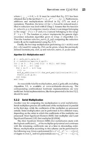
Algorithm 5.5—Multiplication mod f
d := poly_mult_ zp(a,b);
R := reduction_matrix_R_zp(f);
for j in 0 .. m-1 loop c(j) := d(j); end loop;
for j in 0 .. m-1 loop
for i in 0 .. m-2 loop
c(j) :=
mod_m_addition(c(j),dar_mod_multiplication(R(j,i),
d(m+i),p,m),p,m);
end loop;
end loop;
An executable Ada file multiplication_mod_f_poly.adb, including
Algorithm 5.5, is available at www.arithmetic-circuits.org. The
corresponding combinational hardware implementations are very
inefficient. Serial implementations, like those presented in Section 5.2.2,
should be used.

5.2.2 Serial Multiplication
Another way fo r computing the multiplication is serial multiplication.
Serial multipliers process all coefficients of the multiplicand in parallel
in the first step, while the coefficients of the multiplier are processed
serially. Serial multiplication can be performed in two different ways,
depending on the order in which the coefficients of the multiplier are
processed: Most Significant Element (MSE) first multiplier and Least
Significant Element (LSE) first multiplier [GGK06].
The Most Significant Element (MSE) first multiplication starts with
the highest coefficient b of the multiplier polynomial and continues
m − 1
with the remaining coefficients one at a time in descending order.
Hence, multiplication according to this scheme can be performed in
+
m
the following way. Given a polynomial f(x) = x + f x m − 1 . . . + f x + f
m − 1 1 0
+
of degree m over Z , and two polynomials a(x) = a x m − 1 . . . + a x + a
p m − 1 1 0