Page 198 - Hardware Implementation of Finite-Field Arithmetic

m
Operations over GF (2 )—Polynomial Bases 179

irreducible polynomials. Some important irreducible polynomials
will be studied in Sec. 7.6.
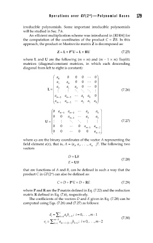
An efficient multiplication scheme was introduced in [RH04] for
the computation of the coordinates of the product C = ZB. In this
approach, the product or Mastrovito matrix Z is decomposed as:

Z = L + P U = L + RU (7.25)
T
where L and U are the following (m × m) and (m – 1 × m) Toeplitz
matric es (diagonal-constant matrices, in which each descending
diagonal from left to right is constant):
⎛ a 0 0 0 0⎞
⎜ a 0 a 0 0 0 ⎟
⎜ a 1 a 0 a 0 0 ⎟
0
L = ⎜ ⎜ 2 1 ⎟ ⎟ (7.26)
⎜ ⎟
⎜ a m −2 a m −3 a 1 a a 0 0 ⎟
⎝ a ⎜ m 1 a m 2 a 2 a 1 a ⎟
0⎠
−
−
⎛ 0 a a a a ⎞
⎜ m −1 m −2 2 1 ⎟
⎜ 0 0 a m −1 a 3 a 2 ⎟
U = ⎜ ⎟ (7.27)
⎜ 0 0 0 a a ⎟
⎜ m −1 m−2 ⎟
−
⎜0 0 0 0 a m − ⎠ ⎟
⎝
1
where a s are the binary coordinates of the vector A representing the
i
field element a(x), that is, A = (a , a , . . . , a ) . The following two
T
0 1 m - 1
vectors
D = LB
(7.28)
E = UB
that are functions of A and B, can be defined in such a way that the
product C in GF(2 ) can also be defined as:
m
T
C = D + P E = D + RE (7.29)
where P and R are the P matrix defined in Eq. (7.22) and the reduction
matrix R defined in Eq. (7.6), respectively.
The coefficients of the vectors D and E given in Eq. (7.28) can be
computed using Eqs. (7.26) and (7.27) as follows:

i ∑
d = i a b − ; i = 0, ... , m−1
k =0 k i k (7.30)
i ∑
e = m = −2 a m−−( k i − ) b k +1 ; i = 0, ... , m −2
+
1
ki