Page 260 - Hardware Implementation of Finite-Field Arithmetic

240 Cha pte r Ei g h t

Therefore, we have the following:
c = a b + a b + a b + a b + a b + a b + a b + a b + aab
3 2 2 3 2 2 3 3 1 1 3 3 0 0 3 1 0 01
c = a b + a b + a b + a b + a b + a b + a b + aab + ab
2 1 1 2 1 1 2 2 0 0 2 2 3 3 2 03 30
c = a b + a b + a b + a b + a b + a b + aab + a b + ab (8.11)
1 0 0 1 0 0 1 1 3 3 1 1 2 21 32 2 3
c = a b + a b + a b + a b + a b + a b + ab + a b + ab
a
0 3 3 0 3 3 0 0 2 2 0 0 1 10 2 1 12
Comparing Eq. (8.11) to Eqs. (8.6) and (8.8), the function h is given by
h a a a a ,
, ,
c = (, , 2 3 ; b b b b , )
2
1
3
3
0
1
0

= ab + a b + a b + ab + a b + ab + ab + a b + ab (8.12)
22 3 2 2 2 3 3 1 1 3 3 0 0 3 1 0 0 1
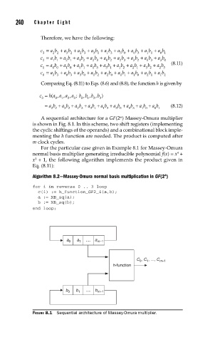
m
A sequential architecture for a GF(2 ) Massey-Omura multiplier
is shown in Fig. 8.1. In this scheme, two shift registers (implementing
the cyclic shiftings of the operands) and a combinational block imple-
menting the h function are needed. The product is computed after
m clock cycles.
For the particular case given in Example 8.1 for Massey-Omura
4
normal basis multiplier generating irreducible polynomial f(x) = x +
x + 1, the following algorithm implements the product given in
3
Eq. (8.11):
Algorithm 8.2—Massey-Omura normal basis multiplication in GF(2 )
4
for i in reverse 0 .. 3 loop
c(i) := h_function_GF2_4(a,b);
a := NB_sq(a);
b := NB_sq(b);
end loop;

a 0 a 1 .... a m–1

C , C , ..., C m–1
0
1
h-function

b 0 b 1 .... b m–1

FIGURE 8.1 Sequential architecture of Massey-Omura multiplier.