Page 264 - Hardware Implementation of Finite-Field Arithmetic

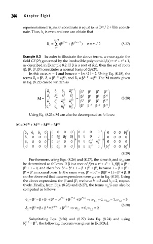
244 Cha pte r Ei g h t

representation of δ , its ith coordinate is equal to its (( /m 2 + )) i th coordi-
v
nate. Thus, h is even and one can obtain that
v
h /2
v ∑
+
δ = v β ( 2 w vk , + β 2 w vk v ) v = m/ 2 (8.27)
,
k=1
Example 8.3 In order to illustrate the above terms, we use again the
4
4
3
field GF(2 ) generated by the irreducible polynomial f(x) = x + x + 1,
as described in Example 8.2. If β is a root of f(x), then the set of roots
{β, β , β , β } constitutes a normal basis of GF(2 ).
8
4
4
2
In this case, m = 4 and hence v = ⎣m/2⎦ = 2. Using Eq. (8.18), the
terms δ = β , δ = β 12 = β , and δ = β 12 2 = β . The M matrix given
+
+
5
2
3
0 1 2
in Eq. (8.22) can be written as
⎛ δ δ δ δ ⎞ β ⎛ 2 β 3 β 5 β ⎞
3
2
9
⎜ δ 0 δ 1 2 δ 2 2 δ 1 2 ⎟ ⎜ 3 4 6 10⎟
⎟
M = ⎜ 1 0 1 2 2 = ⎜ β β β β ⎟ (8.28)
⎜ δ δ 2 δ 2 2 δ ⎟ ⎜ β 5 β 6 β β 8 β 12 ⎟
2
⎜ 2 1 0 1 2 ⎟ β ⎝ 9 β 10 β 12 β ⎠
16
δ ⎝ 2 3 δ 2 δ δ 2 2 δ ⎠
3
1 2 1 0
Using Eq. (8.23), M can also be decomposed as follows:
M = M 0 ( ) + M ( ) + M () + M ()
2
3
1
δ ⎛ ⎛ δ δ 0⎞ ⎛0 0 0 0⎞ ⎛00 0 0 ⎞ ⎛ 0 0 0 δ 2 3 ⎞
⎜ δ 0 1 2 ⎟ ⎜ 0 δ 2 δ 2 δ 2⎟ ⎜ 00 0 0 ⎟ ⎜ 1 ⎟
= ⎜ 1 0 0 0 ⎟ +⎜ ⎜ 0 2 1 2 ⎟ +⎜ 00 δ 2 2 δ 2 2⎟ +⎜ 0 0 0 0 ⎟
⎜ δ 2 0 0 0 ⎟ ⎜ 0 δ 1 0 0 ⎟ ⎜ 0 1 ⎟ ⎜ 0 0 0 0 ⎟
⎜ ⎝ 0⎠ ⎝0 δ 2 0 ⎠ ⎝00 δ 2 2 ⎟ ⎜ 2 3 00 δ 2 ⎟ ⎟
⎟ ⎜
⎟ ⎜
3
δ
⎠
0
0
0
2 0 1 0 ⎠ ⎝ 1 0 ⎠
(8.29)
Furthermore, using Eqs. (8.26) and (8.27), the terms h and w can
j j,k
4
4
3
be determined as follows. If β is a root of f(x) = x + x + 1, f(β) = β +
4
8
2
2
3
β + 1 = 0, and therefore β = β + 1 = β + β + β , because 1 = β + β +
3
β + β in normal basis. In the same way, β = ββ = β(β + 1) = β + β. It
5
8
4
4
3
4
can be observed that these expressions were given in Eq. (8.10). Using
5
the above expressions for β and β , we have h = 3 and h = 2, respec-
3
1 2
tively. Finally, from Eqs. (8.26) and (8.27), the terms w ’s can also be
j,k
computed as follows:
w
w
w
β β +
δ = β = + 2 β = β 2 1 1, + β 2 12, + β 2 13, ⇒ w = 0 w = 1,w = 3
8
3
,
,
1 11 1 12 13
,
,
(8.30)
β
w
w
δ = β 5 = +β 4 = β 2 21, +β 2 2 2, ⇒ w = 0,w = 2
0
,
,
2 21 22
Substituting Eqs. (8.26) and (8.27) into Eq. (8.24) and using
δ 2 i − 1 = β , the following theorem was given in [RH03a].
i
2
0