Page 263 - Hardware Implementation of Finite-Field Arithmetic

m
Operations over GF (2 )—Normal Bases 243

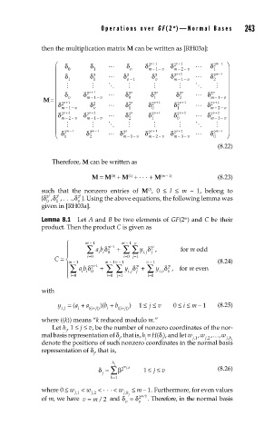
then the multiplication matrix M can be written as [RH03a]:
⎛ δ δ δ δ 2 v + 1 δ 2 v + 2 δ 2 m − 1 ⎞
− − v
1
⎜ 0 1 v m −− v m v + 2 2 1 m − 1 ⎟
⎜ δ 1 δ 2 0 δ 2 v v − 1 δ 2 v δ 2 m − − v δ 2 2 ⎟
1
⎜ ⎟
⎜ δ δ 2 v + 1 δ 2 v δ 2 v δ 2 v δ 2 v ⎟
+
M= ⎜ ⎜ v + 1 v m −− v 0 v 1 v + 1 2 v + 1 m v + −− v⎟ ⎟
1
1
1
⎜ δ 2 m −− v δ 2 v δ 2 1 δ δ 2 0 δ 2 1 δ 2 m −− ⎟
2
1
v
δ ⎜ 2 v + 2 δ 2 v + 2 2 δ 2 v δ 2 v + 1 δ 2 v + 2 δ 2 v + 2 ⎟
−
⎜ m −− v m − 1 v 2 1 0 m −− v ⎟
3
2
⎜ ⎟
⎜ 2 m − 1 1 2 m − 1 2 v 2 v + 1 2 v + 2 2 m − 1 1 ⎟
⎝ δ 1 δ 2 δ m −− δ m − 2 − v δ m − 3 − v δ 0 ⎠
1 v
(8.22)
Therefore, M can be written as
(0)
M = M + M + . . . + M (m − 1) (8.23)
(1)
(l)
such that the nonzero entries of M , 0 ≤ l ≤ m – 1, belong to
{δ 2 l ,δ 2 l , ... ,δ 2 l }. Using the above equations, the following lemma was
0 1 v
given in [RH03a].
m
Lemma 8.1 Let A and B be two elements of GF(2 ) and C be their
product. Then the product C is given as
⎧ m − 1 m − 1 v
i
⎪ ∑ ab δ 2 i−1 + ∑ ∑ y δ , forr m odd
2
⎪ i=0 ii 0 i=0 j=1 i j , j
C = ⎨ m − 1 m − 1 v − 1 v − 1 (8.24)
⎪ ∑ ab δ 2 i 1 + ∑ ∑ y δ + ∑ 2 i
−
i
2
⎪ ii 0 i j , j y δ , for m even
i v v
,
=
=
⎩ i =0 i =0 j=1 i 0
with
y = a ( + a )( b + b ) 1 ≤ j ≤ v 0 ≤ i ≤ m − 1 (8.25)
+
+
ij , i (( i j)) i (( i j))
where ((k)) means “k reduced modulo m.”
Let h , 1 ≤ j ≤ v, be the number of nonzero coordinates of the nor-
j
mal basis representation of δ , that is, h = H(δ ), and let w , w ,… , w
j j j j,1 j,2 j h j
,
denote the positions of such nonzero coordinates in the normal basis
representation of δ , that is,
j
h j
j ∑
δ = β 2 w jk , 1 ≤ j ≤ v (8.26)
k=1
where 0 ≤ w < w < ... < w ≤ m − 1. Furthermore, for even values
j, 1 j, 2 j h j
,
of m, we have v = m/2 and δ = δ 2 m 2 . Therefore, in the normal basis
/
v v