Page 261 - Hardware Implementation of Finite-Field Arithmetic

m
Operations over GF (2 )—Normal Bases 241

where h_function_GF2_4 implements the h function given in Eq. (8.12)
and NB_sq implements normal basis squaring. It must also be noted
that Algorithm 8.2 can be implemented with the sequential architec-
ture given in Fig. 8.1. An executable Ada file NB_seqmult_GF2_4.adb,
including Algorithm 8.2, is available at www.arithmetic-circuits.org.
m
Alternatively, a parallel architecture for a GF(2 ) Massey-Omura
multiplier could be easily implemented [WTSDOR85]. In this scheme,
m identical logic function h that calculate simultaneously all compo-
nents of the product is needed. The inputs of the m logic function h
are connected directly to the components of A and B, as given in
Eq. (8.8). The only difference in the connections to the components of
A and B to a function h is that they are cyclically shifted versions of
one another, as in Eq. (8.8).
m
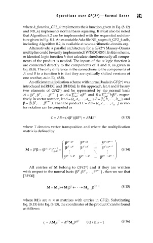
An efficient multiplication scheme with normal basis in GF(2 ) was
introduced in [RH00] and [RH03a]. In this approach, let A and B be any
m
two elements of GF(2 ) and be represented by the normal basis
j
N = {β 2 0 ,β 2 1 , ... , β 2 m − 1 } as A =∑ m − 1 a β 2 i and B =∑ m − 1 b β , respec-
2
i=0 i j=0 j
tively. In vector notation, let A = (a , a , . . . , a m − 1 ), B = (b , b , . . . , b m−1 ), and
1
1
0
0
β β , ...
β = (, 2 β , 2 m − 1 ). Then the product C = AB = (c , c , . . . , c ) in vec-
0 1 m − 1
tor notation can be computed as
T
C = AB = ( Aβ T )(β B ) = AM B T (8.13)
where T denotes vector transposition and where the multiplication
matrix is defined by
⎛ β 2 0 +2 0 β 2 0 +2 1 β 2 0 +2 m − 1 1 ⎞
⎜ β 2 + 2 0 β 2 + 2 1 β 2 + 2 m − 1 ⎟
1
1
1
M = ββ = β( 2 i +2 j m − 1 = ⎜ ⎟ (8.14)
T
)
, ij =0
⎜ ⎟
⎜ β ⎝ 2 m − 1 + 2 0 β 2 m − 1 + 2 1 β 2 m − 1 + 2 m − 1 ⎟ ⎠

m
All entries of M belong to GF(2 ) and if they are written
with respect to the normal basis {β 2 0 ,β 2 1 ,... ,β 2 m − 1 } , then we see that
[RH00]
M = M β + M β + ... + M β 2 m − 1 (8.15)
2
0 1 m − 1
where M ’s are m × m matrices with entries in GF(2). Substituting
i
Eq. (8.15) into Eq. (8.13), the coordinates of the product C can be found
as follows:

c = AM B = A M B i () T 0 ≤ i ≤ m − 1 (8.16)
i ()
T
i i 0