Page 265 - Hardware Implementation of Finite-Field Arithmetic

m
Operations over GF (2 )—Normal Bases 245

m
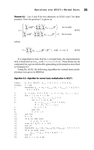
Theorem 8.1 Let A and B be two elements of GF(2 ) and C be their
product. Then the product C is given as
⎧ m − 1 v h h j ⎛ m − 1 ⎞
⎪ ∑ abβ 2 i + ∑∑ ⎜∑ y β 2 i ⎟ , for m odd
⎪ ii (( i − w jk )), j ⎠
,
C = ⎨ i=0 j=1 h k=1 i ⎝ =0 (8.31)
⎪ m 1− 2 i v − 1 j ⎛ m 1− 2 i ⎞
⎪ ∑ abβ + ∑ ∑⎜ ∑ y (( i − w jk )), j j β ⎟ ⎠ + F,forr m even
ii
⎩ i 0= j 1= k 1= ⎝ i 0= ,
where

h / 2 v − 1
v
F = ∑ ∑ y i − (β 2 i + β 2 i + v ) and v = m/ 2 (8.32)
k=1 1 i=0 (( w vk , )), v

It is important to note that for a normal basis, the representation
of δ is fixed and so is w , with 1 ≤ j ≤ v, 1 ≤ k ≤ h . These terms can be
j j,k j
computed for a given irreducible generating polynomial as described
in Example 8.3.
Using Eq. (8.32), the following algorithm for normal basis multi-
plication was given in [RH03a]:

m
Algorithm 8.3—Algorithm for normal basis multiplication in GF(2 )
m
Input: A, B ∈ GF(2 ), w , 1 ≤ j ≤ v, 1 ≤ k ≤ h .
j,k j
Output: C = AB
1. Generate y = (a + a )(b + b ), 1 ≤ j ≤ v,
i,j i ((i+j)) i ((i+j))
0 ≤ i ≤ m-1
2. c := a b , 0 ≤ i ≤ m – 1, C := (c , c ,..., c )
i i i 0 1 m-1
3. for j = 1 to v – 1 do
4. T := (t , t ,..., t ) = 0
0 1 m-1
5. for k = 1 to h do
j
6. r := y , 0 ≤ i ≤ m-1,
i ((i-w j,k )),j
R := (r , r ,..., r )
0 1 m-1
7. T := T + R
8. end for
9. C := C + T
10. end for
11. T := 0
12. If m is odd then
13. s := h , t := m
v
14. else s:= h /2, t := m/2
v
15. end if
16. Generate y , = ( a + a (( v i)) )( b + b (( v i)) , ) 0 ≤ i ≤ t-1
+
+
iv i i
17. If m is even then
18. y := y , 0 ≤ i ≤ m/2 – 1
i+v,v i,v
19. end if
20. for k = 1 to s do