Page 275 - Hardware Implementation of Finite-Field Arithmetic

m
Operations over GF (2 )—Normal Bases 255

where NB_exp performs the square-and-multiply exponentiation in
m
normal basis given in Algorithm 8.5 for a field GF(2 ) with values
h and w . An executable Ada file NB_2kary_exp.adb, including
j j,k
Algorithm 8.8, is available at www.arithmetic-circuits.org.

8.5 Inversion
Efforts in developing normal basis multiplicative inversion algo-
m
rithms in finite fields GF(2 ) have produced only a limited number of
choices. The most popular methods for finite field inversion over
GF(2 ) are mainly based on Fermat’s theorem and on Euclid’s algorithm
m
m
[Sun06]. Using Fermat’s theorem, the inverse of an element in GF(2 )
can be found by successive squaring and multiplication. In normal
basis representation of a Galois field, squaring is done by a simple
cyclic shift. Hence, the algorithms based on Fermat’s theorem for
inversion mainly choose this basis ([IT88], [Fen89], [WTSDOR85]).
m
From Fermat’s theorem, that is, A 2 − 1 = 1, A 2 m = A holds. There-
fore, the inversion can be carried out by computing the exponentia-
tion A −1 = A 2 m − 2 , for A ≠ 0 ∈ GF(2 ). Since 2 – 2 = 2 + 2 + 2 + . . . + 2 m − 1 ,
m
2
3
m
−1
A can be expressed as ([WTSDOR85], [TYT01])
A −1 = A 2 m − 2 = A ( 2 1 )( A )( A )... A ( 2 m − 1 ) (8.37)
2
3
2
2
As stated, squaring can be realized in normal basis representation
by a cyclic shift operation.
The following algorithm [WTSDOR85] implements the inversion
given in Eq. (8.37):
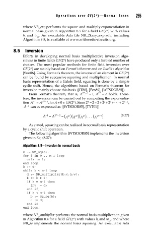
Algorithm 8.9—Inversion in normal basis
b := NB_sq(a);
for i in 0 .. m-1 loop
c(i) := 1;
end loop;
k := 0;
while k < m-1 loop
d := NB_multiplier(b,c,h,w);
k := k + 1;
if k = m-1 then
inv := d;
end if;
if k < m-1 then
b := NB_sq(b);
c := d;
end if;
end loop;
where NB_multiplier performs the normal basis multiplication given
m
in Algorithm 8.4 for a field GF(2 ) with values h and w , and where
j j,k
NB_sq implements the normal basis squaring. An executable Ada