Page 280 - Hardware Implementation of Finite-Field Arithmetic

260 Cha pte r Ei g h t

optimal normal basis can be constructed if p = 2m + 1 is prime and if
either of the above two conditions also holds.
Complexities of the arithmetic operations studied in previous sec-
tions can be further reduced when optimal normal are considered. For
example, the multiplication scheme given in Eq. (8.24), Lemma 8.1,
can be optimized when Type-I optimal normal basis is used as given
below [RH03a].
As stated, a Type-I optimal normal basis is generated by the roots of
+
m
an irreducible AOP. The AOP f(x) = x + x m − 1 . . . + x + 1 is irreducible if
m + 1 is prime and 2 is primitive modulo m + 1. Thus, the roots of an AOP,
j
2
β , with j = 0, 1, . . . , m – 1, form a Type-I optimal normal basis if and only
if m + 1 is prime and 2 is primitive modulo m + 1. The terms δs, with 1 ≤
j
j ≤ m/2, can be determined in this case by ([RH02], [RH03a])
⎧ ⎧ β 2 k j , j = 12,... , m 2 1
−
⎪
,
/
δ = ⎨ (8.39)
j = ∑ m − 1 2 i
/
⎪ 1 i=0 β , j = m 2
⎩
where k can be obtained from
j
2 +≡ k j m+ 1) (8.40)
j
1 2 mod (
It must be noted that there exists a unique k , 0 ≤ k < m, establish-
j j
ing that Eq. (8.40) holds. Substituting Eq. (8.39) into Eq. (8.24) leads to
the following expression of the product C [RH03a]:
⎛ m − 1 ⎞ v−1 ⎛ m − 1 ⎞ 2 k j ⎛ v − 1 ⎞
C = ⎜∑ a bβ 2 i ⎟ ∑ ⎜∑ y β 2 i ⎟ + ⎜ ∑ y iv⎟ (8.41)
+
i ⎝ =0 ii ⎠ j j=1 i ⎝ =0 ij , ⎠ ⎝ i=0 , ⎠
where the right most summation results in 0 or 1, represented in nor-
mal basis by (0, 0, . . . , 0) and (1, 1, . . . , 1), respectively.
Using Eq. (8.41), the following algorithm for Type-I optimal nor-
mal basis multiplication was given in [RH03a]:

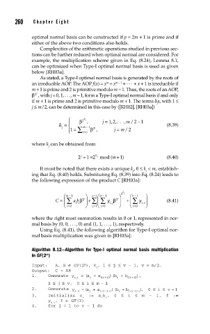
Algorithm 8.12—Algorithm for Type-I optimal normal basis multiplication
m
in GF(2 )
m
Input: A, B ∈ GF(2 ), k , 1 ≤ j ≤ v – 1, v = m/2.
j
Output: C = AB
1. Generate y , = ( a + a (( i j)) )( b + b (( i j)) ),
+
+
ij i i
1 ≤ j ≤ v, 0 ≤ i ≤ m - 1
2. Generate y = a + a )( b + b , ) 0 ≤ i ≤ v– 1
(
i,v i ((v+i)) i ((v+i))
3. Initialize c := a b , 0 ≤ i ≤ m – 1, f :=
i i i
y , f ∈ GF(2)
0,v
4. for j = 1 to v – 1 do