Page 325 - Hardware Implementation of Finite-Field Arithmetic

An Example of Application—Elliptic Curve Cryptography 305

10.5.1 Computation Resources
The computation primitives for executing the elliptic-curve operations
m
are: addition, multiplication, division, and squaring over GF(2 ). The
first one amounts to the component-by-component addition of the
corresponding polynomials. The corresponding circuit is made up of
m XOR gates, and its computation time is equal to 1 clock cycle. For
multiplying, the generic interleaved_mult.vhd model of Chap. 7 (Sec.
7.1.2) can be used. For dividing, a simplified version of binary
Algorithm 6.5, adapted to the case where p = 2, is described in App. C.
The corresponding generic model is binary_algorithm_polynomials.vhd.
Appendix C also includes a specific algorithm for squaring over
163
GF(2 ). The corresponding model is square_163_7_6_3.vhd.
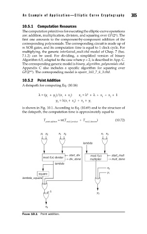
10.5.2 Point Addition
A datapath for computing Eq. (10.16)

2
λ = (y + y )/(x + x ) x = λ + λ + x + x + 1
1 2 1 2 3 1 2
y = λ(x + x ) + x + y
3 1 3 3 1
is shown in Fig. 10.1. According to Eq. (10.69) and to the structure of
the datapath, the computation time is approximately equal to

T ≈ m(T + T ) (10.72)
point-addition mod-f-product mod-f-division

y 1 y 2 x 1 x 2 x 1 x 3

lambda

start_div mod f(x) start_mult
mod f(x) divider
div_done multiplier mult_done
lambda
x 3
y
square 1
lambda_square

1 y 3

x 3

FIGURE 10.1 Point addition.