Page 187 - Innovations in Intelligent Machines

State Estimation for Micro Air Vehicles 179
where V a is the airspeed of the UAV. Bernoulli’s theorem states that [8]

P s = P I + P O ,
where P s is the total pressure, and P O is the static pressure.
Therefore, the output of the differential pressure sensor is

y diff pres = P s − P O + η diff pres
1 2
= ρV + η diff pres (t),
a
2
where η diff pres is a zero mean Gaussian process with known variance.
The static and differential pressure sensors are analog devices that are
sampled by the on-board processer. We will assume that the sample rate is
given by T s .

2.4 GPS
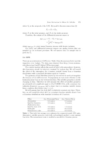
There are several sources of GPS error. Table 1 lists the sources of error and the
respective error budget. The data was obtained from http://www.montana.
edu/places/gps/lres357/slides/GPSaccuracy.ppt.
The current weather affects the speed of light in the atmosphere. However,
this inaccuracy should be relatively constant for a given day. We will model
the effect of the atmosphere by a random variable drawn from a Gaussian
distribution with a standard deviation equal to 5 meters.
The geometry of the Satellites viewed by the receiver is used to triangulate
the location of the GPS receiver. Triangulation is much more effective in the
horizontal plane than in the vertical direction. The satellite geometry is slowly
changing in time. Therefore we will measure the effect of satellite geometry
√
as a sinusoid with amplitude equal to 2.5 2 (RMS=2.5), with a constant but
unknown frequency ω geometry and a phase that is a random variable drawn
from a uniform distribution over [−π, π].
We will assume that the clock drift is relatively constant over time. There-
fore, we will model the clock drift by a constant random variable drawn from
a Gaussian distribution with standard deviation of 1.5 meters.

Effect Ave.HorizontalError Ave.VerticalError
Atmosphere 5.5 meters 5.5 meters
Satellite Geometry 2.5 meters 15 meters
(Ephemeris) data
Satellite clock drift 1.5 meters 1.5 meters
Multipath 0.6 meters 0.6 meters
Measurement noise 0.3 meters 0.3 meters
Table 1. This table lists average error estimates for commercial grade GPS units.
Atmosphere, satellite geometry, clock drift, and multipath produce a near constant
bias term. The measurement noise is modeled as an additive Gaussian process