Page 190 - Innovations in Intelligent Machines

182 R.W. Beard
200 500
p n q
100 0
0 - 500
0 5 10 15 20 25 0 5 10 15 20 25
100 50
p e r
50 0
0 - 50
0 5 10 15 20 25 0 5 10 15 20 25
1740 50
h φ
1720 0
1700 - 50
0 5 10 15 20 25 0 5 10 15 20 25
20 50
θ
V a
10 0
0 - 50
0 5 10 15 20 25 0 5 10 15 20 25
100 200
p ψ
0 0
- 100 - 200
0 5 10 15 20 25 0 5 10 15 20 25
time (sec) time (sec)
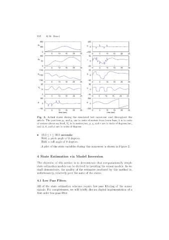
Fig. 2. Actual states during the simulated test maneuver used throughout the
article. The positions p n and p e are in units of meters from home base, h is in units
of meters above sea level, V a is in meters/sec, p, q,and r are in units of degrees/sec,
and φ, θ,and ψ are in units of degrees

• 13.0 ≤ t ≤ 30.0 seconds:
Hold a pitch angle of 0 degrees.
Hold a roll angle of 0 degrees.
A plot of the state variables during this maneuver is shown in Figure 2.

4 State Estimation via Model Inversion

The objective of this section is to demonstrate that computationally simple
state estimation models can be derived by inverting the sensor models. As we
shall demonstrate, the quality of the estimates produced by this method is,
unfortunately, relatively poor for some of the states.

4.1 Low Pass Filters
All of the state estimation schemes require low-pass filtering of the sensor
signals. For completeness, we will briefly discuss digital implementation of a
first order low-pass filter.