Page 194 - Innovations in Intelligent Machines

186 R.W. Beard
1740
actual
1730 estimated
1720
h (m)
1710
1700
1690
0 5 10 15 20 25

18
actual
16 estimated
14
V (m/s)
a
12
10
8
0 5 10 15 20 25
time (sec)
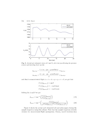
Fig. 5. Actual and estimated values of h and V a after low pass filtering the pressure
sensors and inverting their models

˙ v + ru − pw − g cos θ sin φ
y accel,y = + η accel,y
g
˙ w + pv − qu − g cos θ cos φ
y accel,z = + η accel,z .
g
and that in unaccelerated flight ˙u =˙v =˙w = p = q = r = 0, we get that
C(s){y accel,x } =sin θ

C(s){y accel,y } = − cos θ sin φ
C(s){y accel,z } = − cos θ cos φ.

Solving for φ and θ we get
! C(s){y accel,y } "
ˆ
φ accel = tan −1 (19)
C(s){y accel,z }

ˆ
θ accel = tan −1 C(s){y accel,x } . (20)
2
C(s){y accel,y } + C(s){y accel,z } 2
Figure 6 shows the actual and estimated roll and pitch angles during the
sample trajectory using this scheme. Note that the sample trajectory severely
violates the unaccelerated flight assumptions. Clearly, model inversion does