Page 199 - Innovations in Intelligent Machines

State Estimation for Micro Air Vehicles 191
and f(·) is the probability density function for x i . Given any pair of compo-
nents x i and x j of X, we denote their covariance as
cov(x i ,x j )= Σ ij = E{(x i − µ i )(x j − µ j )}.

The covariance of any component with itself is the variance, i.e.,

var(x i )= cov(x i ,x i )= Σ ii = E{(x i − µ i )(x i − µ i )}.
The standard deviation of x i is the square root of the variance:

stdev(x i )= σ i = Σ ii .
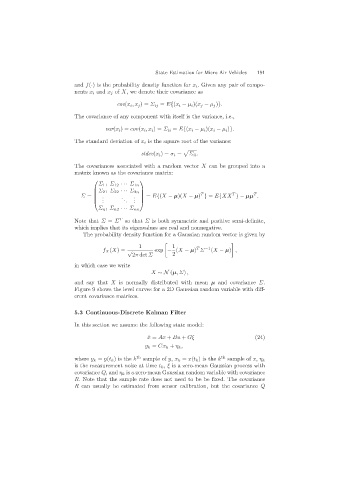
The covariances associated with a random vector X can be grouped into a
matrix known as the covariance matrix:

⎛ ⎞
Σ 11 Σ 12 ··· Σ 1n
Σ 21 Σ 22 ··· Σ 2n T T T
⎜ ⎟
⎜
Σ = ⎜ . . . ⎟ = E{(X − µ)(X − µ) } = E{XX }− µµ .
⎟
⎝ . . . . . . ⎠
Σ n1 Σ n2 ··· Σ nn
Note that Σ = Σ T so that Σ is both symmetric and positive semi-definite,
which implies that its eigenvalues are real and nonnegative.
The probability density function for a Gaussian random vector is given by

1 1 T −1
f X (X)= √ exp − (X − µ) Σ (X − µ) ,
2π det Σ 2
in which case we write
X ∼N (µ,Σ) ,
and say that X is normally distributed with mean µ and covariance Σ.
Figure 9 shows the level curves for a 2D Gaussian random variable with diff-
erent covariance matrices.

5.3 Continuous-Discrete Kalman Filter

In this section we assume the following state model:
˙ x = Ax + Bu + Gξ (24)
y k = Cx k + η k ,

where y k = y(t k )isthe k th sample of y, x k = x(t k )isthe k th sample of x, η k
is the measurement noise at time t k , ξ is a zero-mean Gaussian process with
covariance Q,and η k is a zero-mean Gaussian random variable with covariance
R. Note that the sample rate does not need to be be fixed. The covariance
R can usually be estimated from sensor calibration, but the covariance Q