Page 200 - Innovations in Intelligent Machines

192 R.W. Beard

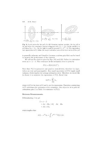
Fig. 9. Level curves for the pdf of a 2D Gaussian random variable. On the left is
the pdf when the covariance matrix is diagonal with Σ 11 <Σ 22. In the middle is a
T
pdf when Σ 22 <Σ 11. On the right is a pdf for general Σ = Σ > 0. The eigenvalues
and eigenvectors of Σ define the major and minor axes of the level curves of the pdf

is generally unknown and therefore becomes a system gain that can be tuned
to improve the performance of the observer.
We will use the observer given by Eqs. (22) and (23). Define the estimation
error as ˜x = x − ˆx. The covariance of the estimation error is given by

T
P(t)= E{˜x(t)˜x(t) }.
Note that P(t) is symmetric and positive semi-definite, therefore its eigen-
values are real and non-negative. Also small eigenvalues of P(t) imply small
variance, which implies low average estimation error. Therefore, we would like
to choose L to minimize the eigenvalues of P(t). Recall that

n

tr(P)= λ i ,
i=1
where tr(P) is the trace of P and λ i are the eigenvalues. Therefore, minimizing
tr(P) minimizes the estimation error covariance. Our objective is to pick the
estimation gain L in Table 3 to minimize tr(P(t)).

Between Measurements.

Differentiating ˜x we get
˙
˜ x =˙x − ˆx ˙
= Ax + Bu + Gξ − Aˆx − Bu
= A˜x + Gξ,
which implies that

t
At
˜ x(t)= e x 0 + e A(t−τ) Gξ(τ) dτ.
˜
0