Page 202 - Innovations in Intelligent Machines

194 R.W. Beard
Plugging back into Eq. (25) give
T
T
T −1
T −1
−
P + = P − + P C (R + CP C ) CP − − P C (R + CP C ) CP −
−
−
−
T −1
T −1
T
T
−
−
+ P C (R + CP C ) (CP C + R)(R + CP C ) CP −
−
−
T
T −1
−
= P − − P C (R + CP C ) CP −
−
T −1
T
−
−
=(I − P C (R + CP C ) C)P −
−
=(I − LC)P .
Extended Kalman Filter.
If instead of the linear state model given in (24), the system is nonlinear, i.e.,
˙ x = f(x, u)+ Gξ (26)
y k = h(x k )+ η k ,
then the system matrices A and C required in the update of the error covari-
ance P are computed as
∂f
A(x)= (x)
∂x
∂h
C(x)= (x).
∂x
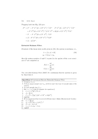
The extended Kalman filter (EKF) for continuous-discrete systems is given
by Algorithm 2.
Algorithm 2 Continuous-Discrete Extended Kalman Filter
1: Initialize: ˆx =0.
2: Pick an output sample rate T out which is much less than the sample rates of the
sensors.
3: At each sample time T out:
4: for i =1 to N do {Propagate the equations.}

5: ˆ x =ˆx + T out f(ˆx, u)
N
6: A = ∂f (ˆx)
T T
∂x
7: P = P + T out AP + PA + GQG
N
8: end for
9: if A measurement has been received from sensor i then {Measurement Update}
10: C i = ∂h i (ˆx)
∂x
T −1
T
11: L i = PC i (R i + C iPC i )
12: P =(I − L iC i)P
13: ˆ x =ˆx + L i (y i − C i ˆx).
14: end if