Page 205 - Innovations in Intelligent Machines

State Estimation for Micro Air Vehicles 197
150
100
p (m)
n actual
50
estimated
0
0 2 4 6 8 10 12 14 16
100
p (m)
e
50
actual
estimated
0
0 2 4 6 8 10 12 14 16
200
χ (deg)
0
actual
estimated
- 200
0 2 4 6 8 10 12 14 16
time (sec)
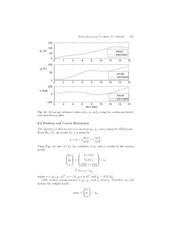
Fig. 11. Actual and estimated values of p n, p e,and χ using the continuous-discrete
extended Kalman filter

6.2 Position and Course Estimation
The objective in this section is to estimate p n , p e ,and χ using the GPS sensor.
From Eq. (3), the model for χ is given by
sin φ cos φ
˙
˙ χ = ψ = q + r .
cos θ cos θ
Using Eqs. (4) and (5) for the evolution of p n and p e results in the system
model
⎛ ⎞
⎛ ⎞ V g cos χ
˙ p N
⎜ ⎟
⎝ ˙p E⎠ = ⎜ V g sin χ ⎟ + ξ p
⎟
⎜
⎝ ⎠
˙ χ q sin φ + r cos φ
cos θ cos θ

= f(x, u)+ ξ p ,
T
T
where x =(p n ,p e ,χ) , u =(V g ,q,r,φ,θ) and ξ p ∼N(0,Q).
GPS returns measurements of p n , p e ,and χ directly. Therefore we will
assume the output model
⎛ ⎞
p n
y GPS = ⎝ p e ⎠ + η p ,
χ