Page 198 - Innovations in Intelligent Machines

190 R.W. Beard
System model:
˙ x = Ax + Bu
y(t k)= Cx(t k)
Initial Condition x(0).
Assumptions:
Knowledge of A, B, C, u(t).
No measurement noise.
In between measurements (t ∈ [t k−1,t k)):
˙
Propagate ˆx = Aˆx + Bu.
+
Initial condition is ˆx (t k−1).
−
Label the estimate at time t k as ˆx (t k).
At sensor measurement (t = t k):

+

−
ˆ x (t k)= ˆx (t k)+ L y(t k) − Cˆx (t k) .
−
Table 3. Continuous-discrete observer for linear time-invariant systems

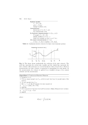
Fig. 8. This figure shows qualitatively the evolution of the state estimate. The
solid line represents the actual state variable and the dashed line represents the
state estimate. Measurements are received at discrete times denoted by t i. Between
measurements, the state estimate is computed by propagating the state model. At
the measurements, the estimate is updated via a weighted average of the current
estimate and the measurement

Algorithm 1 Continuous-Discrete Observer
1: Initialize: ˆx =0.
2: Pick an output sample rate T out which is much less than the sample rates of the
sensors.
3: At each sample time T out:
4: for i =1 to N do {Propagate the state equation.}

5: ˆ x =ˆx + T out (Aˆx + Bu)
N
6: end for
7: if A measurement has been received from sensor i then {Measurement Update}
8: ˆ x =ˆx + L i (y i − C i ˆx)
9: end if

where

E{x i } = ξf i (ξ) dξ,