Page 81 - Innovations in Intelligent Machines

70 P.B. Sujit et al.
x 10 4 q = 1 x 10 4 q = 2
4.5 4 4.5 4
Average total uncertainty 2.5 3 2 Nash Security Average total uncertainty 2.5 3 2 Nash Security
3.5
3.5
Greedy
Greedy
1.5
1.5
Coalition
Cooperative
0.5
0 1 Cooperative 0.5 1 0 Coalition Nash
0 20 40 60 80 100 120 140 160 180 200 0 20 40 60 80 100 120 140 160 180 200
Number of steps Number of steps
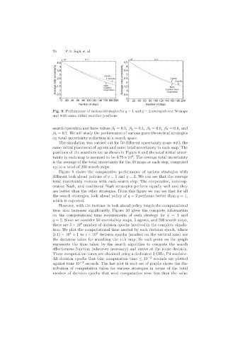
Fig. 9. Performance of various strategies for q = 1 and q = 2 averaged over 50 maps
and with same initial searcher positions

search operation and have values β 1 =0.5,β 2 =0.4,β 3 =0.6,β 4 =0.8, and
β 5 =0.7. We will study the performance of various game theoretical strategies
on total uncertainty reduction in a search space.
The simulation was carried out for 50 different uncertainty maps with the
same initial placement of agents and same total uncertainty in each map. The
positions of the searchers are as shown in Figure 8 and the total initial uncer-
4
tainty in each map is assumed to be 4.75×10 . The average total uncertainty
is the average of the total uncertainty for the 50 maps at each step, computed
up to a total of 200 search steps.
Figure 9 shows the comparative performance of various strategies with
different look ahead policies of q =1 and q = 2. We can see that the average
total uncertainty reduces with each search step. The cooperative, noncoop-
erative Nash, and coalitional Nash strategies perform equally well and they
are better than the other strategies. From this figure we can see that for all
the search strategies, look ahead policy of q = 2 performs better than q =1,
which is expected.
However, with the increase in look ahead policy length the computational
time also increases significantly. Figure 10 gives the complete information
on the computational time requirements of each strategy for q =1 and
q = 2. Since we consider 50 uncertainty maps, 5 agents, and 200 search steps,
4
there are 5 × 10 number of decision epochs involved in the complete simula-
tion. We plot the computational time needed by each decision epoch, where
3
3
(i-1) × 10 +1 to i × 10 decision epochs (marked on the vertical axis) are
the decisions taken for searching the i-th map. So each point on the graph
represents the time taken by the search algorithm to compute the search
effectiveness function (wherever necessary) and arrive at the route decision.
These computation times are obtained using a dedicated 3 GHz, P4 machine.
All decision epochs that take computation time ≤ 10 −3 seconds are plotted
against time 10 −3 seconds. The last plot in each set of graphs shows the dis-
tribution of computation times for various strategies in terms of the total
number of decision epochs that need computation time less than the value