Page 41 - Solutions Manual to accompany Electric Machinery Fundamentals

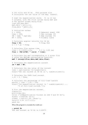
% 240 volts and 50 Hz. This program also
% calculates the rms value of the mag. current.

% Load the magnetization curve. It is in two
% columns, with the first column being mmf and
% the second column being flux.
load p22_mag.dat;
mmf_data = p22(:,1);
flux_data = p22(:,2);

% Initialize values
S = 1000; % Apparent power (VA)
Vrms = 240; % Rms voltage (V)
VM = Vrms * sqrt(2); % Max voltage (V)
NP = 1000; % Primary turns

% Calculate angular velocity for 50 Hz
freq = 50; % Freq (Hz)
w = 2 * pi * freq;

% Calculate flux versus time
time = 0:1/2500:1/25; % 0 to 1/25 sec
flux = -VM/(w*NP) * cos(w .* time);

% Calculate the mmf corresponding to a given flux
% using the MATLAB interpolation function.
mmf = interp1(flux_data,mmf_data,flux);

% Calculate the magnetization current
im = mmf / NP;

% Calculate the rms value of the current
irms = sqrt(sum(im.^2)/length(im));
disp(['The rms current at 50 Hz is ', num2str(irms)]);

% Calculate the full-load current
i_fl = S / Vrms;

% Calculate the percentage of full-load current
percnt = irms / i_fl * 100;
disp(['The magnetization current is ' num2str(percnt) ...
'% of full-load current.']);

% Plot the magnetization current.
figure(1);
plot(time,im);
title ('\bfMagnetization Current at 240 V and 50 Hz');
xlabel ('\bfTime (s)');
ylabel ('\bf\itI_{m} \rm(A)');
axis([0 0.04 -0.5 0.5]);
grid on;

When this program is executed, the results are

» prob2_5b
The rms current at 50 Hz is 0.22973

35