Page 39 - Solutions Manual to accompany Electric Machinery Fundamentals

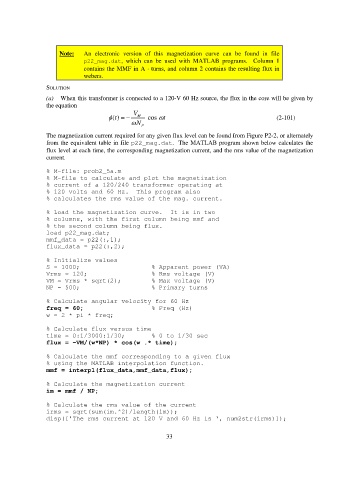
Note: An electronic version of this magnetization curve can be found in file
p22_mag.dat, which can be used with MATLAB programs. Column 1
contains the MMF in A  turns, and column 2 contains the resulting flux in
webers.
SOLUTION

(a) When this transformer is connected to a 120-V 60 Hz source, the flux in the core will be given by
the equation
V
 () t  M cos t  (2-101)
 N P

The magnetization current required for any given flux level can be found from Figure P2-2, or alternately
from the equivalent table in file p22_mag.dat. The MATLAB program shown below calculates the
flux level at each time, the corresponding magnetization current, and the rms value of the magnetization
current.

% M-file: prob2_5a.m
% M-file to calculate and plot the magnetization
% current of a 120/240 transformer operating at
% 120 volts and 60 Hz. This program also
% calculates the rms value of the mag. current.

% Load the magnetization curve. It is in two
% columns, with the first column being mmf and
% the second column being flux.
load p22_mag.dat;
mmf_data = p22(:,1);
flux_data = p22(:,2);

% Initialize values
S = 1000; % Apparent power (VA)
Vrms = 120; % Rms voltage (V)
VM = Vrms * sqrt(2); % Max voltage (V)
NP = 500; % Primary turns

% Calculate angular velocity for 60 Hz
freq = 60; % Freq (Hz)
w = 2 * pi * freq;

% Calculate flux versus time
time = 0:1/3000:1/30; % 0 to 1/30 sec
flux = -VM/(w*NP) * cos(w .* time);

% Calculate the mmf corresponding to a given flux
% using the MATLAB interpolation function.
mmf = interp1(flux_data,mmf_data,flux);

% Calculate the magnetization current
im = mmf / NP;

% Calculate the rms value of the current
irms = sqrt(sum(im.^2)/length(im));
disp(['The rms current at 120 V and 60 Hz is ', num2str(irms)]);

33