Page 47 - Solutions Manual to accompany Electric Machinery Fundamentals

I(1,:) = amps .* ( 0.8 - j*0.6); % Lagging
I(2,:) = amps .* ( 1.0 ); % Unity
I(3,:) = amps .* ( 0.8 + j*0.6); % Leading

% Calculate VS referred to the primary side
% for each current and power factor.
aVS = VP - (Req.*I + j.*Xeq.*I);

% Refer the secondary voltages back to the
% secondary side using the turns ratio.
VS = aVS * (200/15);

% Plot the secondary voltage (in kV!) versus load
plot(amps,abs(VS(1,:)/1000),'b-','LineWidth',2.0);
hold on;
plot(amps,abs(VS(2,:)/1000),'k--','LineWidth',2.0);
plot(amps,abs(VS(3,:)/1000),'r-.','LineWidth',2.0);
title ('\bfSecondary Voltage Versus Load');
xlabel ('\bfLoad (A)');
ylabel ('\bfSecondary Voltage (kV)');
legend('0.8 PF lagging','1.0 PF','0.8 PF leading');
grid on;
hold off;
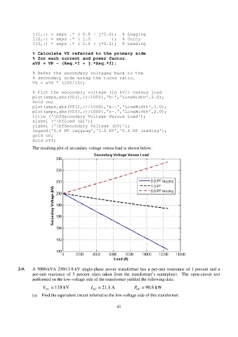
The resulting plot of secondary voltage versus load is shown below:

2-9. A 5000-kVA 230/13.8-kV single-phase power transformer has a per-unit resistance of 1 percent and a
per-unit reactance of 5 percent (data taken from the transformer’s nameplate). The open-circuit test
performed on the low-voltage side of the transformer yielded the following data:

.
V OC  138 kV I OC  21.1 A P  90.8 kW
OC
(a) Find the equivalent circuit referred to the low-voltage side of this transformer.

41