Page 210 - Materials Chemistry, Second Edition

L1644_C05.fm Page 183 Monday, October 20, 2003 12:02 PM

The way to calculate the probability distribution from an enormous amount of
experimental data will be explained here with a brief example:
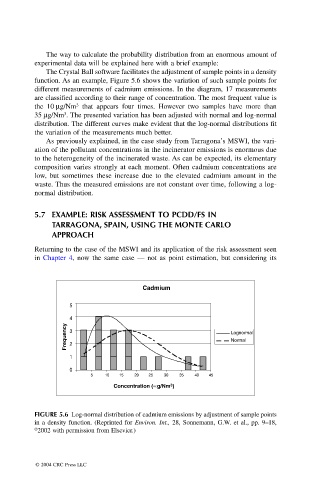
The Crystal Ball software facilitates the adjustment of sample points in a density
function. As an example, Figure 5.6 shows the variation of such sample points for
different measurements of cadmium emissions. In the diagram, 17 measurements
are classified according to their range of concentration. The most frequent value is
3
the 10 mg/Nm that appears four times. However two samples have more than
3
35 mg/Nm . The presented variation has been adjusted with normal and log-normal
distribution. The different curves make evident that the log-normal distributions fit
the variation of the measurements much better.
As previously explained, in the case study from Tarragona’s MSWI, the vari-
ation of the pollutant concentrations in the incinerator emissions is enormous due
to the heterogeneity of the incinerated waste. As can be expected, its elementary
composition varies strongly at each moment. Often cadmium concentrations are
low, but sometimes these increase due to the elevated cadmium amount in the
waste. Thus the measured emissions are not constant over time, following a log-
normal distribution.

5.7 EXAMPLE: RISK ASSESSMENT TO PCDD/FS IN
TARRAGONA, SPAIN, USING THE MONTE CARLO
APPROACH

Returning to the case of the MSWI and its application of the risk assessment seen
in Chapter 4, now the same case — not as point estimation, but considering its

Cadmium

5
4
Frequency 3 Lognormal

Normal
2
1
0
6
5
4
9
8
7
2
1 5 10 15 20 25 30 35 40 45
3
Concentration (µg/Nm 3 )

FIGURE 5.6 Log-normal distribution of cadmium emissions by adjustment of sample points
in a density function. (Reprinted for Environ. Int., 28, Sonnemann, G.W. et al., pp. 9–18,
© 2002 with permission from Elsevier.)
© 2004 CRC Press LLC