Page 249 - Integrated Wireless Propagation Models

M i c r o c e l l P r e d i c t i o n M o d e l s 227

4.3.2.2 Finding the Path Loss Slopes from the Measured Data
The data are stored in corresponding radial zones. The slopes and intercepts are calcu­
lated for each zone and each range, that is 0 to d , d to d , and d to 1 mile. The area
1
1
f f
around the transmitter is typically divided into radial zones, and the zones are typically
uniformly distributed. The Fresnel distance is then calculated for the central radial line
of each zone.
First, if no measured data exist, then as soon as the predicted slopes o f Eq. (4.3.1.1)
y
and1 ofEq. (4.3.2.1.1) are determined, thedistanced canbecalculatedfromEq. (4.3.2.1.4).
1
1
If measurement data do exist, the data are then distributed into corresponding zones.
The data in each zone are then further separated and stored in three ranges: 0 to d d to
f' f
d , and d to 1 mile. We may call each range the sub-zone.
1
1
We may either subtract diffraction loss or add effective antenna height gain in order
to normalize the measured data in each subzone for a flat terrain. When the distance d
between the base station and measured point is less than the near-in distance, only dif­
fraction loss is subtracted. When the distance d is greater than the near-in distance, the
diffraction loss is subtracted and effective height gain added. Diffraction losses and
effective antenna height gain can be calculated at each measurement point. The predic­
tion will start after the normalization of the measurement data.
The line fitting is taken on the normalized measured data in the 0 to d range, and
f
we obtain slope 10 and the power intercept Pd at the near-in distance d Similarly, the
r
f
slope 1 can be found from the line fitting on the normalized measured data in the range
1
from d to d • The slope 1 can be found from the line fitting on the measured data from
1
f
2
1
d to 1 mile (r0 ), as shown in Fig. 4.3. . 1 mostly time 1 can be assumed by y. Since it is
1
2
possible that the lines 10 and 1 do not intersect at Pd at the distance d , we may need to
1
f
f
modify the distance d to be the distance where lines intersect. Similarly, 1 and y gener­
1
f
ate a power intercept at d , at the second breakpoint between d and 1 mile.
1
f
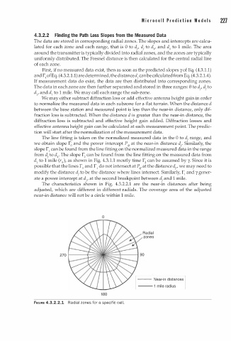
The characteristics shown in Fig. 4.3.2.2.1 are the near-in distances after being
adjusted, which are different in different radials. The coverage area of the adjusted
near-in distance will not be a circle within 1 mile.
0
Radial
zones

•••••••••• Near-in distances

1 8 0
FIGURE 4.3.2.2.1 Radial zones for a specific cell .