Page 247 - Integrated Wireless Propagation Models

M i c r o c e l l P r e d i c t i o n M o d e l s 225

where P,1 = standard radiated power in dBm;
G li = effective antenna height gain in dB, G = 0 for d = d ;
1
,ffi,
ef f
L0 = diffraction loss in dB;
d = distance from transmitter to mobile in meters;
'A = wavelength in meters; and
a = standard adjustments in dB.
D. The received signal in the range d to d assuming that no measured data exist
l
1
'
between d and d , is
1
1
P
P, = Pa -( J�:: }d - d 1 ) in watts for d < d 1 and d s; d s; d 1 (4.3.1.3)
1
1
1
1
1
where Pa is obtained from (4.3.1.2b) at d = d (convert to watts),
1
1
Pa = the signal power received at d (convert to watts),
(pd - pd : 1
J 1 - d f 1 = t he path loss slope in linear scale,
d = distance less than r0, d can be adjusted based on the measured data, and
1
1
d = Fresnel distance in meters.
1
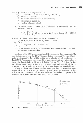
As shown in Fig. 4.3.1.1, this microcell model is composed of three breakpoints. The
near-in distance shown in Eq. (4.3.1.2b) induces the first breakpoint. The second break­
point is determined by Eq. (4.3.1.3), and the last breakpoint is the 1-mile intercept in
Eq. (4.3.1.1). These equations can be used if no measurement data are available. One of
the special characteristics of this model is that the distance d/d s; d s; r0) can be fine­
1
1
tuned based on the measured data. When the measured data are available, the break­
points are calculated and adjusted based on the measured data on a per radial basis.
Also, when the measured data are available in a region, the region around the trans­
mitter will be narrowed to a specific number of radial zones. The measurement data
will be assigned to zones and will be based on finding the best line fitting slope to the
measurement data to achieve each zone's own path loss curve.
0 Editable point
D Fixed point

0.01 d, 0 . 1 d, r0 = 1.0
Distance (miles) (Log scale)

M
e
FIGURE 4.3.1.1 A u l tiple-break point mod l .