Page 400 - Integrated Wireless Propagation Models

378 C h a p t e r S i x

where A is a constant and y is the path-loss exponent. L0 is the loss of the signal strength
from any cause while propagating along the radio path. When in a free space propaga-
tion condition, = (�r and y = 2 and L0 = 0.
A
3
Equation (6.5. . 1 ) is a general equation, that can be represented in all the cell
size-specific path-loss formulas.
The noise power is the sum of all the noise sources:
N = Thermal noise + amplifier noise + human-made noise (6.5.3.2)

The noise figure F is the ratio of two signal-to-noise ratios (SNR), that is (SNR); , and
(SNR) It can be expressed as (SNR); " at the input of a network to (SNR)0111 at the output
out"
2
of the network, as shown in Fig. 6.5.3.1. 8
F = (SNR); " (6.5.3.3)
(SNR) out

where 5; = signal power at the input of the network, such as at the amplifier input port;
N; = noise power at the output of the network, such as at the amplifier output port;
N a = n etwork noise referred to the input of the network, such as the amplifier noise; and
=
G n etwork gain, such as the amplifier gain.
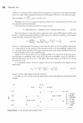
Figure 6.5.3.1 shows that 5/N; is 40 dB and that I N becomes 35 dB after pass­
S
o
ing through an amplifier with a gain of 20 dB and an amplifier noise of 3 dB above
the thermal noise, which is N; = -100 dBm. The noise figure as 5 dB can be found
from Eq. (6.5.3.3).
In a cascaded system shown in Figure 6.5.3.2, the composite noise figure can be
obtained as
F 1 F 1 · · F 1
-
-
- "
F comp = F l +_1.__+ 3 + ·+ (6.5.3.4)
G 1 G G 2 G G
1
1 . . . 11-1
where F" is the noise figure of the nth network.
Usually, we will use the received signal power and noise figure to calculate the link
budget.

t,--- - - - - .-�- - - - -
-40 S 0 = GS;
S; = -60 dBm
-60 --------,.----- S; S0/N0 = 35 dB G = 20 dBm
E N; = -1 00 dBm
co
"0 T N8 = - 97 dBm
-80 S;IN; = 40 dB N0 S0 = -40 dBm
N0 = - 75 dBm
-1 00 N; F = 5 dBm
,
_ __ t
�
L_ _ _ _ _ _ _ _ _ _ _ _ _ _ _ _ _ _ _ _ _ _ _ _ _ _ ime
i
FIGURE 6.5.3.1 S0/N0 after ga n and amplifier noise.