Page 397 - Integrated Wireless Propagation Models

T h e l e e C o m p r e h e n s i v e M o d e l - I n t e g r a t i o n o f t h e T h r e e l e e M o d e l s 375

Macro
Tx
*

Micro Tx � � �
�
�
- - - - �
� 1 2 1 1 .._, ;:, � r--h � 0.87 m
1 4 1i .f. !'• ... p
15 �� i
1 6 • 100 . • 8
Pico Tx 1 7 • 1 Terra1n · • 7 6 I
I
1 8 • 25 ml 1 contour • • I I
DO 20 1 9 • • : 30 m I I
, . � t "
+ - - - - - - - - - - - - - - - �
r1=2200 m
- - - - - - - - - - - - - - - - - - �
r2=2300 m
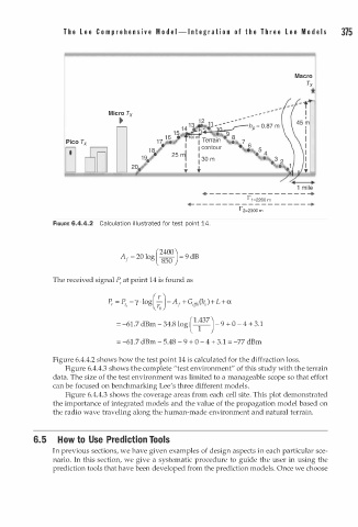
FIGURE 6.4.4.2 Calculation i l lustrated for test point 14.

(2400
A 1 = 20 log ) = 9 dB
850
The received signal P, at point 14 is found as

P, = P , - y · log(�) - A 1 + G, ,(h,) + L + a
ff7
,
1 . 37
= -61.7 dBm - 34.8 log ( { ) - 9 + 0 - 4 + 3.1

0
= -61.7 dBm - 5.48 - 9 + - 4 + 3.1 = -77 dBm
Figure 6.4.4.2 shows how the test point 14 is calculated for the diffraction loss.
Figure 6.4.4.3 shows the complete "test environment" of this study with the terrain
data. The size of the test environment was limited to a manageable scope so that effort
can be focused on benchmarking Lee's three different models.
Figure 6.4.4.3 shows the coverage areas from each cell site. This plot demonstrated
the importance of integrated models and the value of the propagation model based on
the radio wave traveling along the human-made environment and natural terrain.

6.5 How to Use Prediction T o ols
In previous sections, we have given examples of design aspects in each particular sce­
nario. In this section, we give a systematic procedure to guide the user in using the
prediction tools that have been developed from the prediction models. Once we choose