Page 395 - Integrated Wireless Propagation Models

T h e l e e C o m p r e h e n s i v e M o d e l - I n t e g r a t i o n o f t h e T h r e e l e e M o d e l s 373

The effective antenna height he' is measured the height at the base station from the
intercepted point of a line that is drawing from the tip of the hill along the slope of the
hillside to the base station:

A = the frequency offset adjustment in dB = 20 log( { (3.1.2.2)
8 0)
1
a = (gb' - 6 ) + ( g, - 0 ) + 20 log [ ��� ] + 10 log[;�� J
3 5

= !!igb + !!ig, + !!ig,,] + !!ig, 2 (3.1.2.6)
G,ffl,(h.) = 20 log[�'J (no-shadow condition) (3.1.2.3)
,

where h1' and h2' are in meters.
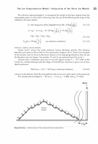
Figure 6.4.4.1 shows the radio distance versus elevation profile. The distance
between each point is 50 m (164 ft). The transmitter height is 45 m. Point 12 is the peak
of the terrain, and it is 30 m in elevation. Note it is not scale proportional so that we can
fit all points into one figure. Two points, 12 and 14, are selected from Fig. 6.4.4. .
1
i
Assume this s suburban area and e use the signal receipt P," = -61 . 7 dBm at the
w
1-mile (or . 6-km) intercept and the slope of 38.4 dB/dec based on a given set of stan­
1
dard conditions:
Path loss = -61.7 - 34.8 log (r /intercept distance) (6.4.4.1)
d
where i s the distance from the transmitter to the receiver in miles and r is the intercept.
0
1
The actual antenna height h/ = 45 m, h ' = . 5 m, gb' = 6 dBd, and g,' = 0 dBd.
z
Macro
Tx

1 2
1 3 ..
1 4 • �
Terrain
contour

..
1 mile
FIGURE 6.4.4.1 Vertical view of the macroce l test environment.
l