Page 55 - Integrated Wireless Propagation Models

I n t r o d u c t i o n t o M o d e l i n g M o b i l e S i g n a l s i n W i r e l e s s C o m m u n i c a t i o n s 33

r------------d------------�

e
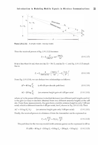
FIGURE 1.9.1.3.1 A simple model-two-ray mod l .

Then the received power f Eq. (1.9.1.3.2) becomes
o
� 2
P - P /.} . 2 4rt h (1.9.1.3.7)
2 2
sm �
r - 0 (4rt) d
If L1<j is less than 0.6 rad, then sin (�<I> /2) "' M /2, cos(�<i>/2) "' l, and Eq. (1.9.1.3.7) simpli­
fies to

(1.9.1.3.8)

From Eq. (1.9.1.3.8), we can deduce two relationships as follows:

d'
�P = 4 0 log j- (a 40-dB-per-decade path loss) (1.9.1.3.9)
I
h'
�G = 2 0 logi;" (an antenna height gain of 6 dB per octal (1.9.1.3.10)

where M is the power difference in decibels between two different path lengths and �G
is the gain (or loss) in decibels obtained from two different antenna heights at the cell
site. From these measurements, the gain from a mobile antenna height is only 3 dB per
octal, which is different from the 6 dB per octal, for h; shown in Eq. (1.9.1.3.10 . Then
)
9
(an antenna height gain only 3 dB per octal) (1. . 1 . 3.11)
Finally, the received power at a distance d from the transmitter can be expressed as

(1.9.1.3.12)

The path loss for the two-ray model (with antenna gains) can be expressed in dB as

PL (dB) = 40log - (10log G1 + 0 l og G"' + 20logh1 + 10log� ) (1.9.1.3.13)
d
1