Page 60 - Integrated Wireless Propagation Models

38 C h a p t e r O n e

k = 3

- - - - - - - - - - - - - - - -
-
- - - - - - - - - - - - -
- - - - - -
- - - - - - - -
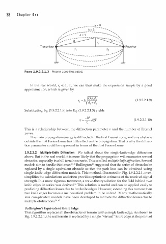
FIGURE 1.9.2.2.1.3 Fresnel zone illustrated.

In the real world, rk « d1 ,d , we can thus make the expression simple by a good
2
approximation, which is given by

(1.9.2.2 1 . 9)
.
Substituting Eq. (1.9.2.2.1.9) into Eq. (1.9.2.2.1.5) yields

(1.9.2.2.1.10)

This is a relationship between the diffraction parameter v and the number of Fresnel
zones.
The main propagation energy is diffracted in the first Fresnel zone, and any obstacle
outside the first Fresnel zone has little effect on the propagation. That is why the diffrac­
tion parameter could be expressed in terms of the first Fresnel zone.

1.9.2.2.2 Multiple-Knife Diffraction We talked about the single-knife-edge diffraction
above. But in the real world, it is more likely that the propagation will encounter several
obstacles, especially in a hill terrain scenario. This is called multiple-knife diffraction. Several
1
models aim to handle this issue.38-4° Bullington4 suggested that the series of obstacles be
replaced by a single equivalent obstacle so that the path loss can be obtained using
single-knife-edge diffraction models. This method, illustrated in Fig. . 9.2.2.2.1, over­
1
simplifies the calculations and often provides optimistic estimates of the received signal
strength. In a more rigorous treatment, a wave-theory solution for the field behind two
knife edges in series was derived.38 This solution is useful and can be applied easily to
predicting diffraction losses due to two knife edges. However, extending this to more than
two knife edges becomes a mathematical problem to be solved. Many mathematically
less complicated models have been developed to estimate the diffraction losses due to
multiple obstructions.39,4 0

Bullington's Equivalent Knife Edge
This algorithm replaces all the obstacles of terrain with a single knife edge. As shown in
1
Fig. . 9.2.2.2.1, the real terrain is replaced by a single "virtual" knife edge at the point of