Page 61 - Integrated Wireless Propagation Models

I n r o d u c t i o n t o M o d e I i n g M o b i I e S i g n a I s i n W i r e I e s s C o m m u n i c a t i o n s 39
t

- - -
---
- - - - - -
- ---

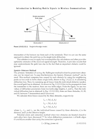
Obstruction 1 Obstruction 2
e
FIGURE 1.9.2.2.2.1 Single-knife-edge mod l .

o
o
w
intersection f the horizon ray from each f the terminals. Then e can use the same
approach to obtain the path loss as the single knife diffraction.
This solution is easy to apply but oversimplifies the calculations and often provides
optimistic estimates of the received signal strength. Therefore, it provides results that
may underestimate the path loss due to the fact that an important obstacle could be
ignored.

Epstein-Peterson Method
The primary limitation of using the Bullington method is that the prominent obsta­
2
cles can be wiped out. To ease this limitation, the Epstein-Peterson method4 can be
used. This method computes loss caused by each obstacle by using the neighboring
peaks as two ends to form a basic single knife, shown in Fig. . 9.2.2.1.1, in calculating
1
diffraction loss. Then, by summing up all losses from the individual obstacles (peaks),
1
the overall path loss is obtained. As shown in Fig. . 9.2.2.2.2(a), in the propagation from
the transmitter to the receiver, there are two knife edges. From the figure, we see two
values of diffraction parameters from two knife-edge heights, h 1 and h • Then the indi­
2
1
vidual diffraction loss is obtained. In Fig. . 9.2.2.2.2(b), there are three obstacles, 01, 02,
and 03, between T (transmitter) and R (receiver).
We calculate three losses caused by the three obstacles, respectively:
, d , h
Lol = f(d l 2 l )
L = f(d A 2 , h )
02
2
L o 3 = f(d d , h )
3' 4 3
where L 01 L , and L are the individual losses caused by three obstacles, d is the
0
02
i
3
'
distance, and h is the effective height.
i
Potential errors and correction method when two obstacles are located closed to
each other have been discussed.43A4 So when diffraction parameters v of both edges
01 and 02 are smaller than unity, the correction is given by
L = 20 log10 (cosec a) (1.9 .2.2.2.1)